ECA Klein-4 Symmetries (Mirror, Complement, Combined)
ECA Klein-4 Symmetries (Mirror, Complement, Combined)
The 256 elementary cellular automata are organized by a Klein-4 group of trivial conjugations:
◼
Mirror — ↔ tape reversal
f(a, b, c) = g(c, b, a)
◼
Complement — ↔ bit complement
f(a, b, c) = ¬g(¬a, ¬b, ¬c)
◼
Composition — apply both
Each is involutive and they commute, so the orbit of any rule has at most four elements. For Rule 110 the orbit is . The two generators give six edges in the universality graph; this notebook proves and visualises all of them as bisimulations with σ = 1, τ = 1.
{110, 124, 137, 193}
Setup
SetEnvironment["PATH"->Environment["PATH"]<>":"<>FileNameJoin[{$HomeDirectory,".elan","bin"}]];PacletDirectoryLoad[FileNameJoin[{NotebookDirectory[],"..","Resources","LeanLink","LeanLink"}]];Get["LeanLink`"];leanProjectDir=FileNameJoin[{NotebookDirectory[],"..","Lean"}];
1. Klein-4 Orbit of an ECA Rule
Each ECA rule is a local map . Wolfram encodes it by listing the outputs for neighbourhoods in that order and reading the resulting 8-bit string as a binary integer. Thus Rule 110 is .
Fin 2 × Fin 2 × Fin 2 → Fin 2
111, 110, 101, 100, 011, 010, 001, 000
01101110
The code below accesses the same rule table in the little-endian order used by : bit is the output on neighbourhood , so the bit positions correspond to .
BitGet
4 a + 2 b + c
(a, b, c)
0, 1, ..., 7
000, 001, ..., 111
Mirror acts by , so it swaps bit positions and , fixing .
(a, b, c) → (c, b, a)
1 ↔ 4
3 ↔ 6
0, 2, 5, 7
Complement acts by , so bit becomes .
f( a, b, c ) → 1 - f( 1 - a, 1 - b, 1 - c )
i
1 - (bit (7 - i) of original)
neighborhoodIndex[a_,b_,c_]:=4a+2b+cwolframNeighborhoods=Tuples[{1,0},3];wolframRuleTable[ruleNumber_Integer]:=BitGet[ruleNumber,neighborhoodIndex@@@wolframNeighborhoods]mirrorRule[ruleNumber_Integer]:=Sum[BitGet[ruleNumber,neighborhoodIndex[c,b,a]]*2^neighborhoodIndex[a,b,c],{a,0,1},{b,0,1},{c,0,1}]complementRule[ruleNumber_Integer]:=Sum[(1-BitGet[ruleNumber,neighborhoodIndex[1-a,1-b,1-c]])*2^neighborhoodIndex[a,b,c],{a,0,1},{b,0,1},{c,0,1}]orbit[ruleNumber_Integer]:=DeleteDuplicates@{ruleNumber,mirrorRule@ruleNumber,complementRule@ruleNumber,mirrorRule@complementRule@ruleNumber}
orbit[110]
{110,124,137,193}
Expected: .
{110, 124, 137, 193}
Row[{"Rule 110 in Wolfram order: ",wolframRuleTable[110]}]
Rule 110 in Wolfram order: {0,1,1,0,1,1,1,0}
Expected: , corresponding to .
{0, 1, 1, 0, 1, 1, 1, 0}
111, 110, 101, 100, 011, 010, 001, 000
2. Rule Tables Side by Side
littleEndianRuleTable[ruleNumber_Integer]:=Table[BitGet[ruleNumber,i],{i,0,7}]
We display the rule tables in Wolfram's order. The little-endian order remains useful for bit manipulations.
111, 110, ..., 000
000, 001, ..., 111
TableForm[Table[wolframRuleTable[r],{r,orbit[110]}],TableHeadings->{orbit[110],Row/@wolframNeighborhoods}]
111 | 110 | 101 | 100 | 011 | 010 | 001 | 000 | |
110 | 0 | 1 | 1 | 0 | 1 | 1 | 1 | 0 |
124 | 0 | 1 | 1 | 1 | 1 | 1 | 0 | 0 |
137 | 1 | 0 | 0 | 0 | 1 | 0 | 0 | 1 |
193 | 1 | 1 | 0 | 0 | 0 | 0 | 0 | 1 |
TableForm[Table[littleEndianRuleTable[r],{r,orbit[110]}],TableHeadings->{orbit[110],Table[Row@IntegerDigits[i,2,3],{i,0,7}]}]
000 | 001 | 010 | 011 | 100 | 101 | 110 | 111 | |
110 | 0 | 1 | 1 | 1 | 0 | 1 | 1 | 0 |
124 | 0 | 0 | 1 | 1 | 1 | 1 | 1 | 0 |
137 | 1 | 0 | 0 | 1 | 0 | 0 | 0 | 1 |
193 | 1 | 0 | 0 | 0 | 0 | 0 | 1 | 1 |
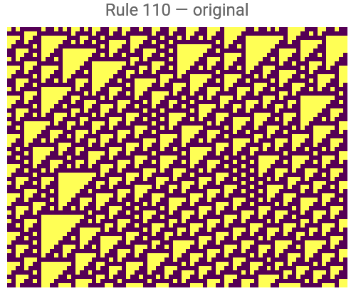
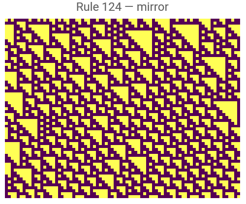
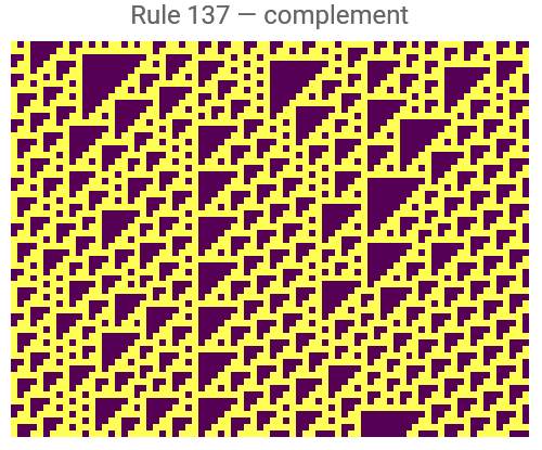
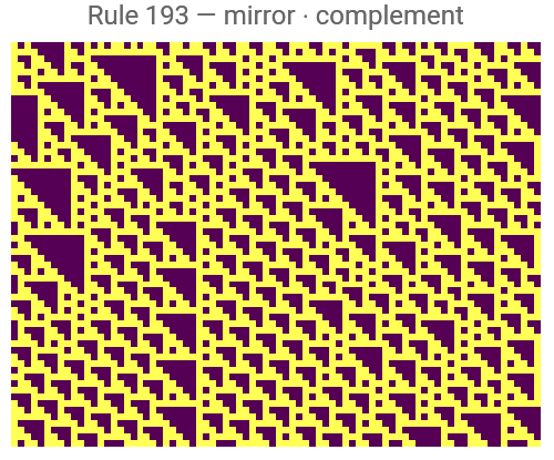
3. Visual Demonstration
We evolve all four rules from the same random initial tape and apply the corresponding tape transforms. The plots should match (up to permutation/inversion) by the conjugation theorems.
init=RandomInteger[1,80];nSteps=60;
plotEvolution[rule_Integer,label_String]:=ArrayPlot[CellularAutomaton[rule,init,nSteps],Frame->False,ImageSize->250,PlotLabel->Style[Row@{"Rule ",rule," — ",label},12],ColorRules->{0->Lighter@Yellow,1->Darker@Purple}]
Grid@{{plotEvolution[110,"original"],plotEvolution[124,"mirror"]},{plotEvolution[137,"complement"],plotEvolution[193,"mirror · complement"]}}
Verifying the conjugations pointwise
Verifying the conjugations pointwise
reverseTape[tape_List]:=Reverse@tapecomplementTape[tape_List]:=1-tapeevolveLast[rule_Integer,tape_List,k_Integer]:=CellularAutomaton[rule,tape,k][[-1]]
Mirror — :
step rule110 (reverse tape) = reverse (step rule124 tape)
And@@Table[evolveLast[110,reverseTape@init,k]===reverseTape@evolveLast[124,init,k],{k,1,nSteps}]
True
Complement — :
step rule110 (complement tape) = complement (step rule137 tape)
And@@Table[evolveLast[110,complementTape@init,k]===complementTape@evolveLast[137,init,k],{k,1,nSteps}]
True
Mirror · Complement — :
step rule110 (reverse · complement tape) = reverse · complement (step rule193 tape)
And@@Table[evolveLast[110,reverseTape@complementTape@init,k]===reverseTape@complementTape@evolveLast[193,init,k],{k,1,nSteps}]
True
All three should return .
True
4. Lean Verification
The point of this section is not just that Lean accepts the file, but that you can inspect the exact claims being proved.
◼
The machine definitions live in .
Lean/Machines/ElementaryCellularAutomaton/Defs.lean
Machine definitions
Machine definitions
The ECA rules are defined literally by their Wolfram numbers:
Klein-group framework (mirror, complement, combined)
Klein-group framework (mirror, complement, combined)
The generic, rule-parametric statements:
Exact edge statements
Exact edge statements
These are the actual no-hypothesis simulation theorems for the Rule 110 orbit edges: