[ LLM Generated ]
Displacements on graphs
Displacements on graphs
Claude Fable 5
Abstract.
A displacement moves every vertex of a finite connected graph to a set of nearby vertices; it is the graph counterpart of the time- flow of a vector field, defined from the shortest-path distance alone. We prove that the sum of displacements is commutative, that for single-valued displacements 1-continuity coincides with nonexpansiveness, that 1-continuous displacements form a monoid graded by magnitude, and that a single-valued bijective 1-continuous displacement is a graph automorphism; on the Cayley graph of a finitely generated abelian group the generator translations commute exactly. Bounding the magnitude by 1 does not make a bijective displacement an automorphism, and a Killing displacement need not have constant pointwise magnitude. On the 8 by 8 honeycomb patch the sum of the two period translations equals the translation by the sum of the periods at graph distance greater than 2 from the boundary, and the bound 2 cannot be lowered.
r
1
.Definitions
Definitions
Definition
1
.1
.Let be a finite connected graph with shortest-path distance . A displacement is a map assigning to every vertex a nonempty set of vertices; its magnitude is
G=(V,E)
d
D
A displacement of scale is a section of the tangent bundle whose fiber over is the ball of radius at . A value set with more than one element records a tie which the metric does not break.
r
v
r
v
Remark
1
.2
.A displacement is set-valued by default, and we do not reserve a separate name for the single-valued case. The reason is that the single-valued displacements are not closed under the operations defined below. Only composition preserves single-valuedness; the sum, the inverse, the scaling and the commutator of two single-valued displacements are in general multivalued, as the computation below shows. A convention under which "displacement" meant the single-valued object would therefore name a class which the theory leaves after one operation. We keep "displacement" for the set-valued object, write "single-valued displacement" where the special case is meant, and call a single-valued displacement contained in a given one a selection of it. The same convention applies to the other infrageometric notions, where ties in the metric are the rule and not the exception.
Example
1
.3
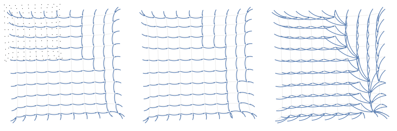
.Two random single-valued displacements on each of the six example graphs, put through the five operations; the entry is the largest value set in the result. Composition stays single-valued on every graph; each of the other four operations produces a multivalued result on at least one graph — the sum on the grid, the triangular patch and the disc, the commutator on the grid, the inverse on the grid and the disc, the scaling on four of the six graphs. Below the table, the grid case is drawn: the two reduced random displacements and their sum; a tie shows as two arcs leaving the same vertex.
compose | sum | commutator | inverse | scale | |
cycle | 1 | 1 | 1 | 1 | 1 |
grid | 1 | 2 | 6 | 3 | 3 |
triNbhd | 1 | 2 | 1 | 1 | 5 |
cayley | 1 | 1 | 1 | 1 | 1 |
disc | 1 | 2 | 1 | 2 | 3 |
hexGrid | 1 | 1 | 1 | 1 | 2 |
Definition
1
.4
.A displacement is k-continuous when for every edge some pair of targets is at distance at most :
D
u∼v
k
Definition
1
.5
.The composition of displacements applies the flows left to right and collects targets over every intermediate point: the value of ∘ at is the union of (w) over .
D
2
D
1
v
D
2
w∈(v)
D
1
Definition
1
.6
.The sum of two displacements is the bisector of the two composition orders,
m
By the Baker–Campbell–Hausdorff formula the two orders realise the sum plus and minus half the commutator, so their midpoints realise the sum with the commutator cancelled, to third order in the scale.
Definition
1
.7
.The inverse of a displacement reflects every step through its base point — the scale minus-one case of scaling. The scaling moves to the endpoints of geodesics from through its targets, rescaled to times their length:
tD
v
v
t
where runs over the aligned candidates: those on a geodesic ray through the target — the opposite ray for negative — and among candidates at the best rounded distance the straightest are kept, those carried by the most geodesics.
c
t
Definition
1
.8
.The commutator of two displacements is the group commutator of the flows, with inverses taken as reflections:
It is second order in the scale, which is why a first-order object like the bracket is necessarily scale-dependent on a graph.
Definition
1
.9
.A Killing displacement is a single-valued displacement that is a graph automorphism. The reduction of a displacement contracts every value set toward its metric centre — the members of least eccentricity under the mutual distances — iterated to a fixed point.
Definition
1
.10
.The pointwise magnitude of a displacement at a vertex is the largest distance from to a target, . The magnitude of is the maximum of over . Call constant if is constant on , and varying otherwise. The vertices with are the fixed points of .
D
v
v
r(v)=d(v,w)
max
w∈D(v)
D
r
V
D
r
V
r(v)=0
D
Construction
1
.11
.Four displacements exist on every graph and recur below. The polar pair at a centre: the radial displacement steps outward along the geodesics from the centre, the angular displacement steps along the cross edges of constant distance; a vertex with no admissible step stays put, and the angular displacement is two-valued wherever both rotation senses exist. The gradient displacement of a vertex function moves every vertex to the neighbours where the function increases most; local maxima stay put. The translation displacement along an embedding moves every vertex to the vertices whose coordinates are nearest to its own position shifted by a given vector. The random displacement of scale is built by breadth-first shell extension with repair sweeps, aiming at 1-continuity.
k
Example
1
.12
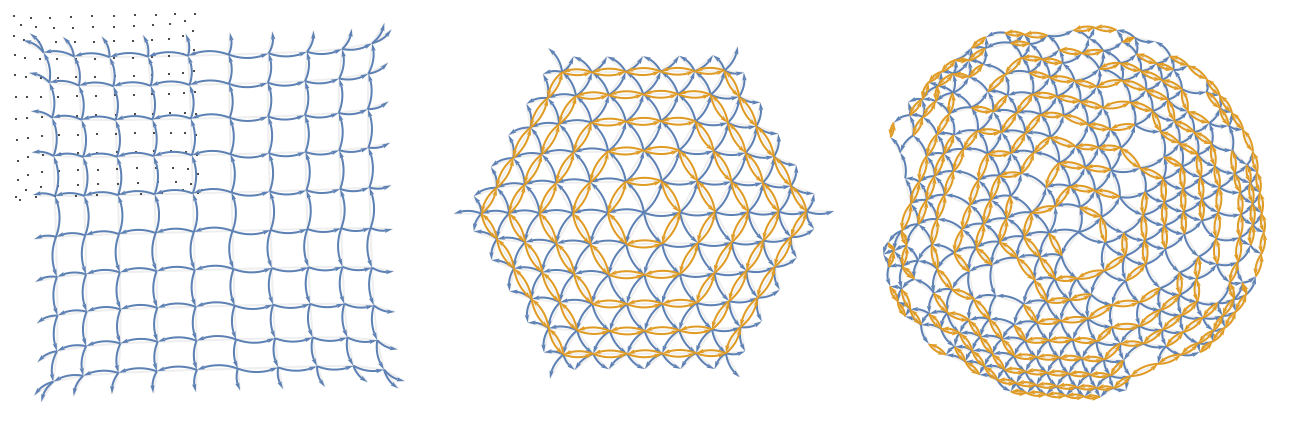
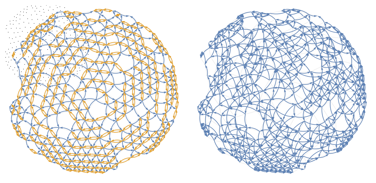
.1-continuity of the constructions across the six example graphs, at scale 1, with the horizontal coordinate as the function for the gradient. The radial displacement is 1-continuous on the five regular graphs and fails on the irregular disc mesh; the angular displacement fails also on the triangular patch; the gradient displacement is 1-continuous on none of the six; the random displacement is 1-continuous on all six. The polar pair is drawn on the grid, the triangular patch and the disc mesh, and on the disc the composite of the radial and the angular displacement is a discrete spiral.
radial | angular | gradient | random | |
cycle | True | True | False | True |
grid | True | True | False | True |
triNbhd | True | False | False | True |
cayley | True | True | False | True |
disc | False | False | False | True |
hexGrid | True | True | False | True |
2
.Classification and structure
Classification and structure
Remark
2
.1
.Write for single-valued, for bijective, for 1-continuous and for Killing. On every finite connected graph : the forward implication holds since an automorphism is bijective and nonexpansive, the converse is . The magnitude and the distinction between constant and varying are independent of all four predicates: the magnitude grades the monoid of 1-continuous displacements (), but bounding it implies none of , , , , and neither does it follow from them. The two observations give the counterexamples.
S
B
C
K
K⇔S⋀B⋀C
S
B
C
K
Observation
2
.2
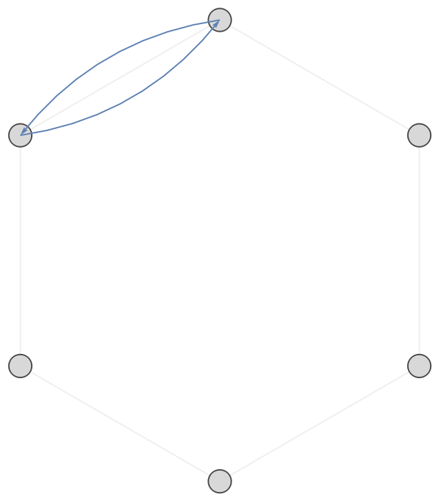
.Bounding the magnitude by 1 does not imply continuity, and hence does not imply that a bijective displacement is an automorphism. A transposition along an edge moves each of two adjacent vertices onto the other and fixes the rest; it is single-valued, bijective and of magnitude 1, but it is not 1-continuous and not an automorphism. On the six-cycle it collapses the distance between the vertices 1 and 3 from 2 to 1.
Example
2
.3
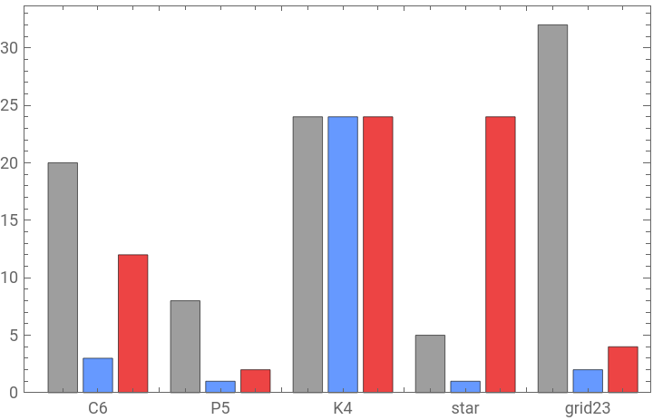
.The edge transposition on the six-cycle, and the count over all permutations of five small graphs: the permutations of magnitude at most 1, those of them which are automorphisms, and all automorphisms. On the six-cycle only 3 of the 20 permutations with magnitude at most 1 are automorphisms, so the magnitude bound is much weaker than continuity. On the star the automorphisms (24) exceed the magnitude-1 permutations (5), so automorphisms need not have magnitude 1 either; on all three counts coincide at 24, since the diameter is 1.
K
4
{True,True,1,False,False}


Observation
2
.4
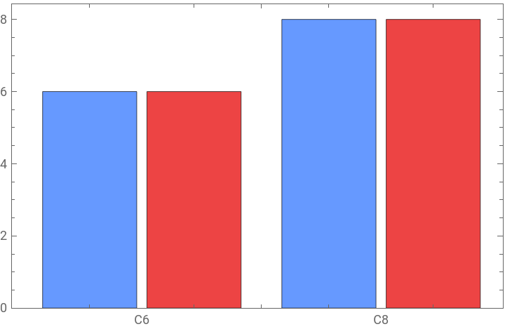
.Constancy is independent of the predicates as well. Among the 12 automorphisms of the six-cycle, the 6 rotations (including the identity) have constant pointwise magnitude and the 6 reflections do not — a reflection fixes an axis and moves the remaining vertices by up to the diameter. The split is again half and half, 8 against 8, on the eight-cycle.
Example
2
.5
.Constant against varying pointwise magnitude over all automorphisms of the six- and eight-cycle, and the pointwise magnitude of a rotation against a reflection of the six-cycle.


Example
2
.7
.Random 1-continuous displacements on each of the six example graphs; the entry records whether the two sums agree exactly.
Proposition
2
.10
.The composite of two 1-continuous displacements is 1-continuous, and magnitudes are subadditive:
Example
2
.11
.Composites of two random scale-2 displacements on each of the six example graphs; the check combines 1-continuity of the composite with subadditivity.
Proposition
2
.12
.A single-valued bijective 1-continuous displacement of a finite connected graph is a graph automorphism.
Proof.
A nonexpansive bijection of a finite metric space permutes the multiset of pairwise distances while not increasing any, so it preserves them all; a distance-preserving bijection of a connected graph maps edges to edges.
□
Proposition
2
.14
.On the Cayley graph of a finitely generated abelian group the generator translations are Killing displacements and all their pairwise commutators are the identity displacement.
Proof.
Right multiplication by a generator is an automorphism of the Cayley graph; for abelian groups the four flows of the group commutator cancel pointwise.
□
Observation
2
.16
.The least magnitude of a nontrivial Killing displacement is not always 1: it is 1 on the ten-cycle and on the abelian Cayley graph, 2 on the interior grid, 7 on the triangular patch and 14 on the honeycomb patch. The two patches admit only patch symmetries — automorphism groups of order 12 and 4 — whose elements displace vertices by up to the patch diameter. The disc mesh is omitted: its automorphism group is trivial, so it admits no nontrivial Killing displacement at all.
Example
2
.17
.The least magnitude of a nontrivial Killing displacement on the five example graphs that admit one; below, the minimal Killing displacement is drawn on the ten-cycle, the interior grid and the triangular patch — magnitudes 1, 2 and 7.
Example
2
.19
.The two period translations and their sum, drawn on the honeycomb patch; then the vertices where the sum equals the diagonal translation, in green — the vertices where they differ, in red, lie along the boundary. The two booleans are the margin-2 and margin-1 statements.
Claim
2
.20
.The breadth-first repair construction of the random displacement does not always return a 1-continuous displacement: on the honeycomb patch at scale 3 with seed 3, eleven edges violate the continuity condition.
Example
2
.21
.The scale-3 random displacement on the honeycomb patch and, next to it, its eleven violating edges highlighted.
3
.Questions
Questions
4
.References
References
[Hall2015]
Hall, Brian C., Lie Groups, Lie Algebras, and Representations: An Elementary Introduction, 2015
[BuragoBuragoIvanov2001]
Burago, Dmitri and Burago, Yuri and Ivanov, Sergei, A Course in Metric Geometry, 2001
5
.Symbols
Symbols
Constructions:
Operations:
Invariants and predicates:
◼
DisplacementSingleValuedQ — every value set is a single vertex
◼
DisplacementBijectionQ — the induced map is a bijection
Visualisation:
◼
DisplacementPlot — bent arcs over the graph's own embedding