[ LLM Generated ]
Displacements on graphs
Displacements on graphs
Claude Fable 5
Abstract.
A displacement is a set-valued metric flow on a graph. Composition gives a relation monoid with a subadditive magnitude, while the continuous bijective part is the group of graph isometries. Metric negatives and relation inverses give two different commutator loops, selected explicitly by method; the examples use a 140-vertex grid, a 127-vertex triangular neighborhood, and a 100-vertex uniform-length disc.
1
.Definitions
Definitions
Definition
1
.1
.Let be a finite connected graph. A displacement is a map , with pointwise magnitude (v)=d(v,w) and global magnitude
G=(V,E)
D:V⟶𝒫(V)
r
D
max
w∈D(v)
Values remain sets: a metric tie is geometric data, not a choice of representative.
Example
1
.2
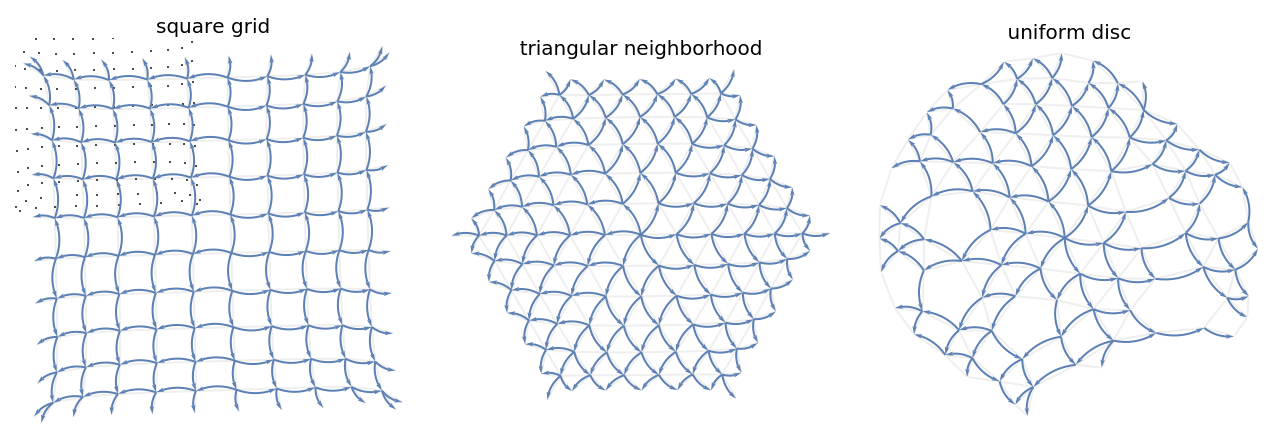
.Outward radial displacements on three larger graph substrates:
Definition
1
.3
.The identity displacement is . Composition acts leftmost first,
I(v)={v}
For a scalar , consists of endpoints obtained by continuing the geodesics , , to distance nearest . The negative is .
t
tD
v⟶w
w∈D(v)
td(v,w)
-D=(-1)D
Example
1
.4
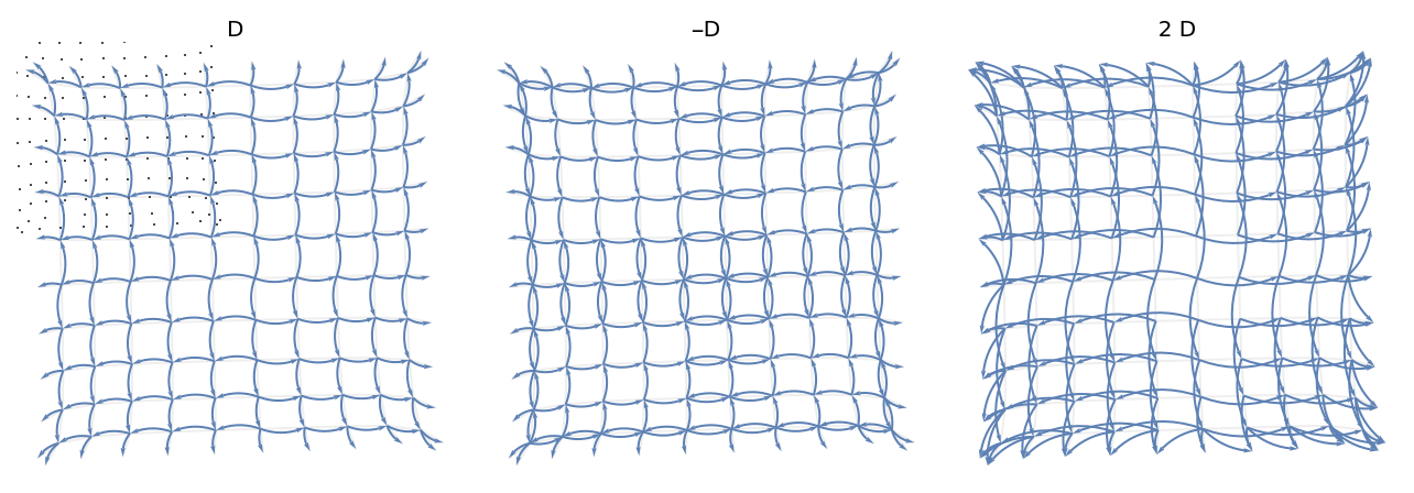
.A radial field, its metric negative, and its double on the 140-vertex grid:
Definition
1
.5
.The inverse is the inverse relation,
-1
D
It is a map inverse exactly when is bijective. The reduction iterates the metric center operation on every value set, retaining every tied center.
D
ρ(D)
Example
1
.6
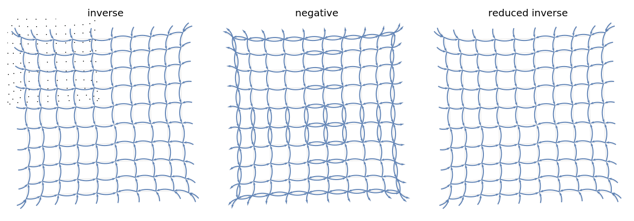
.Relation inverse and metric negative use different geometry on the radial field; the former collects fibers, while the latter reflects arrows through their source vertices:
Definition
1
.7
.The sum + is the set of metric midpoints between the two composition orders ∘ and ∘. It is the metric counterpart of cancelling the quadratic commutator terms in the Baker-Campbell-Hausdorff comparison .
D
1
D
2
D
2
D
1
D
1
D
2
Example
1
.8
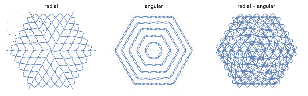
.The radial and angular fields on the triangular neighborhood have a nontrivial metric sum:
Definition
1
.9
.For finite sets , write
A,B⊆V
A displacement is respectively weakly, Hausdorff, or strongly -continuous when the chosen distance between and is at most for every edge .
k
D(u)
D(v)
k
uv
Definition
1
.10
.A Killing displacement is a single-valued graph isometry. Its least nonzero magnitude is the Killing displacement magnitude; it is when the graph has no nonidentity automorphism.
∞
Definition
1
.11
.At a center , the radial and angular displacements move respectively along and across the distance spheres of . A gradient displacement follows neighbors maximizing a vertex function, and a translation displacement follows a graph embedding. samples a continuous displacement of prescribed magnitude.
c
d(c,·)
RandomDisplacement
Example
1
.12
.The triangular radial field is the gradient of its distance function, while its angular companion follows the distance spheres:
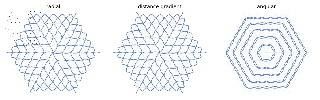
Definition
1
.13
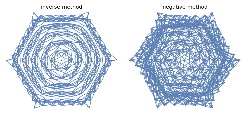
.There are two commutator loops. The inverse method is
which is the exact group commutator when both displacements are bijections. The negative method is
the metric loop at the scale of the two fields. selects them with or ; is the negative-method shorthand.
DisplacementCommutator
Method->"Inverse"
Method->"Negative"
DisplacementBracket
Example
1
.14
.The two loops of the radial and angular fields differ on the triangular neighborhood because relation inverse and metric negative are different operations:
2
.Algebraic and metric structure
Algebraic and metric structure
Proposition
2
.1
.Displacements of form a monoid under composition, with identity . Their magnitude is subadditive:
G
I
Proof.
Relation composition is associative. For , , and , the graph triangle inequality gives ; maximizing over all three vertices gives the bound.
v∈V
u∈(v)
D
1
w∈(u)
D
2
d(v,w)≤d(v,u)+d(u,w)
□
Proposition
2
.2
.Weakly -continuous displacements form a submonoid. The magnitude therefore grades the continuous relation monoid by the preceding subadditivity inequality.
1
Proof.
Across an edge choose a close pair of first-step targets, then a close pair of second-step targets. The resulting composite targets are again at graph distance at most one.
□
Proposition
2
.3
.The metric sum is exactly commutative:
Proof.
Swapping the two fields interchanges the two composition orders and leaves their midpoint set unchanged.
□
Proposition
2
.4
.A bijective weakly -continuous displacement of a finite graph is a graph isometry. Thus the continuous bijective displacements form the Killing group of .
1
G
Proof.
A bijective -Lipschitz map does not increase any pairwise graph distance. It permutes the finite multiset of all pairwise distances, so every inequality is equality; distance one is preserved in both directions.
1
□
Remark
2
.5
.The inverse method belongs to the Killing group when its inputs do. The negative method requires neither bijectivity nor relation inversion and is therefore the metric operation to examine under graph refinement; it is not asserted here to satisfy the Lie identities before such a limit is constructed.
3
.Questions and directions
Questions and directions
Question
3
.1
.On Riemannian-like uniform-length meshes, how do the errors in associativity, scaling, and the negative commutator depend on the displacement magnitude and mesh scale?
Question
3
.2
.Which geometric conditions make the negative commutator anticommutative after rescaling, and which conditions identify its continuum limit with a Lie bracket?
Question
3
.3
.When does metric-center reduction commute with scaling, sum, or composition? In particular, which graph geometries make every relevant midpoint and geodesic continuation unique?
Question
3
.4
.How should boundary effects be separated from intrinsic geometry? The least nontrivial Killing magnitude is large on finite tessellation patches even when their interior has translation-like fields.
Question
3
.5
.Which families of radial, angular, gradient, and translation displacements recover enough first-order data to approximate a tangent bundle under refinement?
Remark
3
.6
.The immediate computations are scaling studies on uniform-length meshes, comparison of regular patches with irregular discs, and classification of the tie sets retained by sum, negative, and reduction.
4
.References
References
The sum is motivated by the Baker-Campbell-Hausdorff comparison .
[Hall2015]
Hall, Brian C., Lie Groups, Lie Algebras, and Representations: An Elementary Introduction, 2015
5
.Symbols
Symbols
Operations:
Predicates and invariants:
Constructions and visualization: