Harmonic oscillator
Harmonic oscillator
A harmonic oscillator is a particle in a potential energy well given by kx², where k is the a positive constant (elastic constant).
V(x)=
1
2
In[]:=
ClearAll["Global`*"](*Thedimensionsoftheimagesproducedareset:400isthewidthand200istheheight.*)MyImageSize={400,200};
In[]:=
$Assumptions=x∈Reals&&(*VariablePositiononthexaxis*)p∈Reals&&(*VariableMomentum*)ℏ∈Reals&&ℏ>0&&(*Planckconstant*)m∈Reals&&m>0&&(*Massoftheparticle*)n∈Integers&&n>0&&(*Integerfornumberofsolutions*)k∈Reals&&k>0&&(*Elasticconstantofthespring*)ω∈Reals&&ω>0(*Pulsationrate*);
SolutionsoftheSchröedingerequation: φ1(x),φ2(x),φ3(x)
SolutionsoftheSchröedingerequation: (x),(x),(x)
φ
1
φ
2
φ
3
In this notebook, for simplicity, we do not solve the Schröedinger equation but we immediately write the solutions and show that they satisfy the Schröedinger equation .
The Schröedinger equation is solvable only for the discrete values of the Energy En[n], they are all possible values for energy. Each solution φ (n, x) represents a physical state and it is associated with its respective energy En[n] .
The Schröedinger equation is solvable only for the discrete values of the Energy En[n], they are all possible values for energy. Each solution φ (n, x) represents a physical state and it is associated with its respective energy En[n] .
We define the angular frequency:
In[]:=
ω=;
k
m
The energy levels numbered with n=0,1,2,3..
In[]:=
En[n_]:=ℏωn+;
1
2
Each solution φ (n, x) represents a physical state and it is associated with its respective energy En[n] .
In[]:=
φ[n_,x_]:=n!HermiteHn,x
1
n
2
1
4
mω
πℏ
-
mω
2
x
2ℏ
mω
ℏ
Solution for n = 1
In[]:=
φ[1,x]//Simplify
Out[]=
2
-
km
2
x
2ℏ
3/8
(km)
1/4
π
3/4
ℏ
Solution for n = 2
In[]:=
φ[2,x]//Simplify
Out[]=
-
km
2
x
2ℏ
1/8
(km)
km
2
x
2
1/4
π
5/4
ℏ
Solution for n = 3
In[]:=
φ[3,x]//Simplify
Out[]=
-
km
2
x
2ℏ
3/8
(km)
km
2
x
3
1/4
π
7/4
ℏ
The elastic potential V (x) written as a function of angular frequency ω:
In[]:=
V[x_]:=m;
1
2
2
ω
2
x
The(x)satisfytheSchroedingerequationforeachvalueofn,trytochangethevalueofn=0,1,2,3,...
φ
n
In[]:=
n=1;-φ[n,x]+V[x]φ[n,x]==En[n]φ[n,x]//FullSimplify
2
ℏ
2m
∂
x
∂
x
Out[]=
True
The(x)arenormalizedforeachvalueofn,trytochangethevalueofn=0,1,2,3,...
φ
n
In[]:=
n=1;x1
∞
∫
-∞
2
Abs[φ[0,x]]
Out[]=
True
Mean value of x is zero for each value of n, try to change the value of n = 0, 1, 2, 3, ...
In[]:=
n=1;=xx
x
+∞
∫
-∞
2
Abs[φ[n,x]]
Out[]=
0
In order to create the graphs, let' s fix the value of the following three constants
In[]:=
ℏ=1;m=1;k=0.1;
Wedefinethefollowingfunctiontodrawthegraphsofrealfunction(x)
φ
n
In[]:=
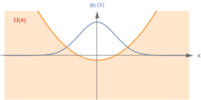
MainColorPlot=ColorData[97,"ColorList"][[1]];GeneratePlot1[En_,f_,fLabel_]:=Plot[{2f,V[x]-En},{x,-9,9},PlotRange{-1.5,1.5},PlotStyle->{Default,Orange},Filling{2->Bottom},Ticks{None,None},AxesStyleDirective[Thickness[0.003],Arrowheads[{0.04}]],AxesLabel{"x",Style[fLabel,MainColorPlot]},PlotPoints100,Epilog{Text[Style["U(x)",Red],{-7.5,1.2}]},BaseStyle12,ImageSizeMyImageSize,AspectRatioFull];
Note that the potential has several different heights for each graph because each value of n corresponds to a different value of the energy En[n]
In[]:=
GeneratePlot1[En[0],φ[0,x],"(x)"]GeneratePlot1[En[1],φ[1,x],"(x)"]GeneratePlot1[En[2],φ[2,x],"(x)"]
φ
0
φ
1
φ
2
Out[]=
Out[]=

Out[]=

In[]:=
Note that the potential has several different heights for each graph because each value of n corresponds to a different value of the energy En[n]
The ProbP functions are the probability density of the momentum p, for any given n=0,1,2.
As in the case of the classical particle, the mean value of p is zero