Being able to solve larger scale PDEs comes at a cost of a longer solution time as will be explained later in this tutorial.
Reducing memory consumption of PDE solving
Load the package:
In[2]:=
Needs["FEMAddOns`"]
The following is an example of how DecompositionNDSolveValue, which implements a domain decomposition method, uses less memory than NDSolve when solving the Poisson equation over a Menger mesh.
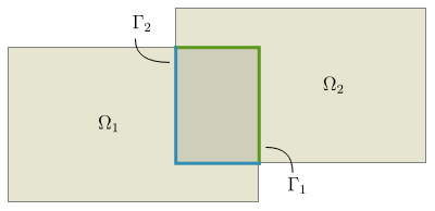
Domain decomposition methods work by dividing the computational region into subdomains. The PDE under consideration is then solved on these subdomains and the solution on the original region is stitched together from the solutions of the subdomains. The memory consumption when computing the solution will never be larger than what it is when solving the problem over the largest subdomain.
The savings in memory come at the price of computational time.
The domain decomposition method is also advantageous because the PDE can be solved simultaneously over the subdomains; not necessarily on the same workstation. For example, a computer cluster can be used by assigning one subdomain to each server.
To solve a PDE, three pieces of information need to be given. A PDE, its boundary conditions, and a region (domain) over which the PDE is to be solved. Consider the following decomposition of the one-dimensional domain
a<x<b
, and how domain decomposition methods can be used to solve a PDE with it.
The figure gives an intuition for why, at least in this case, the convergence rate of Schwarz methods is dependent on the size of the overlap. More generally, one might have subdomains in a higher dimension. For example:
We specify a model PDE that will be used in this section.
Set up a model PDE:
The multiplicative and additive Schwarz methods
DecompositionNDSolveValue implements the multiplicative Schwarz method and the additive Schwarz method for sequential evaluation. They both have robust convergence and the same decrease in the amount of memory, but multiplicative Schwarz has a better convergence rate and is therefore faster when used sequentially (i.e. no kernels have been provided). The additive Schwarz method is inherently parallel, and it is currently the only algorithm available when using the Kernels option to solve problems in parallel.
Solve the equations with additive Schwarz and multiplicative Schwarz:
Make a table comparing the solutions:
The example shows that multiplicative Schwarz and additive Schwarz consume the same amount of memory, but that multiplicative Schwarz is faster.
Adjusting the tolerance of the convergence criterion
DecompositionNDSolveValue stops iteration when the norm falls below the given tolerance:
Providing an approximate solution to speed up convergence
The computations can be sped up by making the Schwarz algorithm converge faster. There are two way to achieve a faster convergence:
The better of an approximation of the actual solution that can be provided, the fewer iterations will have to be done to satisfy the tolerance criterion. The following example shows how to provide an initial guess.
Create a mesh and a coarse version of that mesh:
Find the solution using the coarse mesh:
Count the number of iteration until convergence:
Count the number iterations it takes for the solution to converge when starting from the solution obtained using the coarse mesh:
The example shows that providing an estimate of the solution can decrease the number of iterations required for the solution to converge and therefore decrease the amount of time it takes to solve the problem. The code makes use of the function SetMaxCellMeasure, which takes a mesh and its corresponding symbolic region and creates a new, coarser mesh. It does this by pruning nodes in the body of the mesh while leaving the boundary nodes as they are, thus ensuring that the new mesh covers exactly the same space as the original mesh.
Solving problems in parallel using local or remote kernels
Solve a problem in parallel using two local kernels:
The additive Schwarz method is always used when kernels are provided, because it is very well suited as a parallel domain decomposition method. A parallel version of multiplicative Schwarz has not been implemented in this version. DecompositionNDSolveValue will divide the domain into as many subdomains as there are kernels. If subdomains are specified then the number of kernels should match the number of subdomains. DecompositionNDSolveValue cannot be used with fewer kernels than subdomains, if there are more kernels than subdomains then only the required number of kernels will be used. The subdomains are setup on one kernel each. Each kernel is responsible for solving the PDE over its subdomain once every iteration. The first kernel in the list is matched with the first subdomain in the list and so on. This could be used to place a particularly large subdomain on a computer with more memory. Using a different number of kernels than subdomains will give an error message.
Monitoring the convergence of the solution
The option EvaluationMonitor can be used to evaluate a function after each iteration. The function is given as its first argument the current estimate of the solution and as its second argument the previous estimate of the solution. This can be used to, for example, visualize the progress of the solution, or to compute the norm of the difference between the two arguments to see how far away the norm is from dropping below the specified tolerance.
Monitor convergence using EvaluationMonitor:
The example shows how the norm decreases iteration by iteration until it drops below the tolerance threshold.
Passing subdomain options to DecompositionNDSolveValue
More information can be found in the documentation for ElementMeshDecomposition below.
DecompositionNDSolveValue options
The following table summarizes the options available for DecompositionNDSolveValue.
The currently available domain decomposition methods work for stationary, elliptic partial differential equations in one, two, and three dimensions. As a rule of thumb, any steady partial differential equation that the FEM package can solve, can also be solved with the Schwarz algorithms. Currently, only additive Schwarz is supported for solving PDEs in parallel.
The following example demonstrates that domain decomposition methods can handle equations with convection.
Set up the equation:
Solve convection-diffusion equation using NDSolve:
Solve convection-diffusion equation using DecompositionNDSolveValue:
Compare solutions:
The class of supported PDEs is not limited to systems of equations with one dependent variable as in the previous examples. This makes it possible to use the Schwarz algorithms for solving problems in, for example, structural mechanics. In the following problem, a force is pulling at the edge of a metal plate:
Set up the equations:
Solve the coupled PDEs using DecompositionNDSolveValue:
The convergence rate of one-level Schwarz algorithms, which is the kind of Schwarz algorithms currently implemented, is known to deteriorate with an increasing number of subdomains. The reason is that subdomains only exchange information with their nearest neighbors.
Problem setup:
Solve the problem using NDSolve:
Solve the problem using 2 subdomains, overlap 4, and 50 iterations:
Solve the problem using 5 subdomains, overlap 4, and 50 iterations:
Solve the problem using 10 subdomains, overlap 4, and 50 iterations:
The previous examples show that 50 iterations yield a much better solution when there are fewer subdomains. This is because the convergence rate decreases with an increasing number of subdomains. The convergence rate can be improved in two ways; by increasing the amount of overlap, or by providing a better initial guess.
Solve the problem using 10 subdomains, overlap 20, and 50 iterations:
Solve the problem using 10 subdomains, overlap 4, and 50 iterations, with an initial guess:
Monitoring convergence
Specifying a method for LinearSolve
Set up equations:
Solve the PDE using default solver:
Solve the PDE using "Pardiso":
The smaller memory consumption means that it almost always makes sense to use Pardiso when trying to decrease memory consumption using domain decomposition methods.
Subdomains
The preceding sections have talked about how to solve PDEs using domain decomposition methods. The details of how domains are decomposed into parts, subdomains, has not been discussed as it has been handled by DecompositionNDSolveValue. Sometimes it can be useful to decompose the element mesh separately without using DecompositionNDSolveValue. For example, to check what the subdomains look like, to inspect their properties, or even to implement custom domain decomposition methods. ElementMeshDecomposition is a function that takes an element mesh and returns a decomposition of that element mesh into subdomains. The subdomains can be queried to find information about the subdomain mesh properties and the relationships between the subdomains in terms of for example shared incidents, artificial boundary incidents, and physical boundary incidents. Subdomains returned by ElementMeshDecomposition can be given to DecompositionNDSolveValue in place of a region.
Creating subdomains using ElementMeshDecomposition
Any element mesh can be divided into subdomains using the ElementMeshDecomposition function.
Decompose a rectangle into two subdomains and visualize them:
ElementMeshDecomposition has two options: "Subdomains" and "Overlap". Overlap is the number of layers one subdomain reaches into the neighboring subdomain. In the following example, four layers of elements overlap, which is two layers in each direction from the boundary in between the subdomains in the preceding example. That is, two layers in each direction from the boundary in between the corresponding nonoverlapping subdomains.
Specify two layers of elements of overlap:
"Subdomains" specifies how many subdomains the region should be decomposed into. If an integer is given then ElementMeshDecomposition will attempt to split the element mesh into that many subdomains. If a list of fractions is given then it will try to decompose the element mesh into as many subdomains as there are elements in the list, each with approximately the specified fraction of the total area.
Decompose a Menger mesh into four subdomains with six layers of overlap:
The figure shows four subdomains. The overlapping regions are given distinct colors as well.
Use a list of fractions to divide an element mesh into subdomains of different sizes:
In the preceding example, the blue subdomain takes up roughly 60 % of the area, the yellow subdomain takes up roughly 30 % and the green subdomain takes up roughly 10 %. Subdomains of unequal sizes can be used to distribute the computational load unevenly across kernels if, for example, one kernel has access to more memory than another.
Set overlap as a fraction of the subdomain element graph diameter
Consider an undirected graph representing the connections between elements in a subdomain element mesh. It turns out that the convergence rate is related to the overlap as a percentage of the graph diameter. It is often easier to specify the amount of overlap as a fraction of the graph diameter than as a number of layers because of this. This can be done.
Set the overlap to 10 % of the graph diameter
Use the same overlap specification for a mesh with more subdomains
Use the same overlap specification for a mesh with more mesh elements
The examples show that specifying the overlap as a fraction of the subdomain graph diameter is a good way of ensuring that the overlap will adapt if the number of elements in the subdomains changes.
Specifying overlap for subdomains individually
The subdomains used so far have all extended themselves into their neighbors by approximately same number of layers. It is also possible specify the number of layers for each subdomain individually.
Set overlap to zero for the subdomains in the middle, 20 for the ones at the edge:
One-dimensional and three-dimensional examples
It is not just two-dimensional domains which can be decomposed by ElementMeshDecomposition, but also one-dimensional and three-dimensional domains.
Decomposing a one-dimensional domain into subdomains:
Decomposing a three-dimensional domain into subdomains:
Subdomain wireframe visualization
"Wireframe" accepts the following options, which are the same for subdomains as it is for ElementMesh:
Any options accepted by Graphics will also be applied to the wireframe.
Using the ImageSize option of Graphics to set the size of the resulting graphics:
Specify an edge color for all elements regardless of subdomain:
Lists can be used to specify different options for different subdomains. The list will repeat itself cyclically if the number of stylings in the list is shorter than the number of subdomains.
Style specifications are reused cyclically:
Subdomain data structures
The structure of the object returned by ElementMeshDecomposition is SubdomainGroup[mesh, {Subdomain[...], Subdomain[...], ...}] where mesh corresponds to the global domain. The Subdomain and SubdomainGroup objects have properties. These properties can be used to implement custom domain decomposition methods. They are listed below.
The corresponding incidents in the global mesh are given by the following properties. This is the same as applying the mapping given by LocalToGlobal to the local incidents.
Global versus local incidents
Because each subdomain has fewer incidents than the full mesh the subdomain incidents do not match up with the list of coordinates in the full mesh. This means that two sets of incidents are needed to, say, map the solution vector of a subdomain onto the solution vector of the full mesh. Each type of incident is therefore provided both as local incidents and global incidents. A map is also provided which maps local incidents into global incidents.
Create two subdomains:
Find the coordinates of the artificial boundary using a global mesh:
Find the coordinates of the artificial boundary using a subdomain mesh:
The difference between the first way of getting the boundary incidents and the second is that the incidents are retrieved using the GlobalArtificialBoundaryIncidents property in the first example, and ArtificialBoundaryIncidents in the second example. As always, incidents correspond to coordinates, but in this case they correspond to coordinates in different element mesh objects. The list GlobalArtificialBoundaryIncidents corresponds to coordinates in the full mesh and ArtificialBoundaryIncidents corresponds to elements in the local mesh. In the next example it is shown how incidents retrieved using ArtificialBoundaryIncidents can be converted into incidents that can be used with the coordinates of the full mesh.
How to convert local incidents into global incidents:
Problem setup:
Extract subdomain mesh properties:
Initialize local and global solution vectors:
Extract incident data from subdomains:
Implementation of the Alternating Schwarz method:
Compare solution with NDSolve:
Visualize the solution using ElementMeshInterpolation and Plot3D:
Possible issues
DecompositionNDSolveValue may not be able to solve some PDEs with discontinuous coefficients.