Recurrence Quantification Analysis
Recurrence Quantification Analysis

An analysis method for dynamical systems.
Flip Phillips
Skidmore College Vision Laboratories
© 2015-9
Skidmore College Vision Laboratories
© 2015-9
Introduction
Introduction
Recurrence Quantification Analysis or RQA is a technique for understanding real-world dynamical systems. It consists of three main steps:
◼
Dimensional re-embedding (not strictly a part of the technique, but frequently practiced)
◼
Recurrence map generation
◼
Quantification of map features
Examples
Examples
Preliminaries
Preliminaries
Load the package:
In[]:=
<<RQA`
If you’d like to see what is there —
In[]:=
?RQA`*
Out[]=
Data
Data
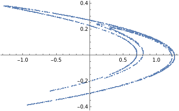
We generate a Henon attractor as example:
In[]:=
α=1.4;β=0.3;nMax=2000;settle=40;
In[]:=
henonxy=Drop[RecurrenceTable[{x[n+1]1-α+y[n],y[n+1]βx[n],x[0]==0.0,y[0]==0.0},{x,y},{n,1,nMax+settle},DependentVariables{x,y}],settle];
2
x[n]
In[]:=
ListPlot[henonxy]
Out[]=
Time Series
Time Series
The RQA package uses the Wolfram Language as its data structure. This is primarily since the analysis our lab has used has been in the time domain. Obviously, RQA is not limited to temporal dynamics, so this is a bit of a compromise that creates a class of parametric function in one variable. Future versions might (well, do in our local stuff) support other parameterizations, multidimensional in nature:
In[]:=
hts=TimeSeries[TemporalData[henonxy,{1,Automatic,1},ValueDimensions2]]
Out[]=
TimeSeries

Let’s use an interesting, 200-wide, window:
In[]:=
tStart=1001;w=200;
In[]:=
hw=TimeSeriesWindow[hts,{tStart,tStart+w-1}]
Out[]=
TimeSeries
Make a 1D, x-only version looking at just the changes of the x-variable:
In[]:=
hx=TimeSeries[TemporalData[hw["Values"][[All,1]],{tStart,tStart+w-1,1}]]
Out[]=
TimeSeries
In[]:=
ListLinePlot[hx,AxesNone,Frame->True,AspectRatio.4]
Out[]=
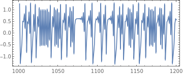
The TimeSeries here assumes a time-step of 1 is equal to an iteration of the attractor. Obviously we are not limited to integer steps or even discrete, equally spaced data. The TimeSeries structure allows us to do all sorts of re-sampling and approximation of the raw data.
Embedding
Embedding
The RQA package has some tools for estimating proper embedding dimension and lag. For now, we’ll simply embed our data into 3 dimensions with a lag/τ of 1.0:
In[]:=
hxe3=RQAEmbed[hx,3,1.0]
Out[]=
TimeSeries
This shows how the x-coordinate jumps back and forth over time but within the pattern of the attractor:
In[]:=
ParametricPlot3D[hxe3[t],{t,1001,1198}]
Out[]=

Distance Map
Distance Map
You can use any distance function you’d like. By default, SquaredEuclideanDistance is used. There are also rescaling options.
The distance map shows distance between a given timestep and all other timesteps during the evolution of the system. In this presentation the x and y axes are increasing t from the lower left. The diagonal is called the LOI or Line of Identity and is always 0 since it is the distance between a point at time t and itself at time t.
Also note that distance maps need not be generated by the RQA package. Any square matrix of distances can be used. It is, of course, up to you to make sure that the map is valid / meaningful.
Recurrence Map
Recurrence Map
Recurrence maps can be generated from two sources — 1) the raw time series, in which case a temporary distance map is generated and destroyed in the process, or 2) from an existing distance map. The former is simpler for quick analyses, the latter for exploration since it doesn’t require the map to be re-computed every time a recurrence map is needed.
Notice that this returns a SparseArray object for space savings and other computational advantages. We can visualize it:
We can also use the previously computed map for efficiency. Here is an interactive example:
Notice that, since the distance map dm is unscaled, we need to describe a different set of controls / thresholds to Manipulate.
Essentially, a recurrence plot indicates locations that, over time, remain within some (usually small) distance. The various structures indicate different properties of the evolving system, namely:
◼
Homogeneity - The process is stable.
◼
Density change in the LL or UR - The process is nonstationary or in transition between states.
◼
White (0) banding - The process is nonstationary with some rare or transitional states.
◼
Periodic patterns - The process has periodic behavior.
◼
Isolated points - The process is dominated by large transitions or may be stochastic.
◼
Diagonal lines parallel to LOI - The process is deterministic in the periodic sense (long lines) or chaotic sense (short lines)
◼
Diagonal lines orthogonal to the LOI - The process is time-reversed or palindromic.
◼
Vertical and horizontal lines and rectangles - The process is ‘laminar’ or stuck.
— From Webber & Zbilut, 2005.
The goal of the following measurements is to describe these qualities in a systematic, quantitative way.
RQA Measurements
RQA Measurements
So - called ‘classical’ RQA consists of five descriptive measures based primarily on the diagonal features of the recurrence map.
Recurrence
Recurrence
Recurrence (aka REC) measures the density of recurrent locations. It describes the relative sparseness of the recurrence map. Small numbers approaching 0 suggest sparseness, numbers approaching 1, denseness.
The RQA package computes exact values for these ratios:
but it is frequently easier to understand these numerically. In early literature, these values were expressed in percentages, so it is advisable to be aware of this.
Determinism
Determinism
Ratio
Ratio
The ratio of REC and DET (RATIO) provides a way of detecting certain transitions. In these cases REC will decrease while the DET remains constant. For our Henon data:
〈D〉
〈D〉
Entropy
Entropy
Entropy (ENT) reflects the complexity of the deterministic structure of the process. High values indicate a more complex system.
Entropy is not systematically related to the length of line segments.
Trend
Trend
The Trend (TND) tells how stationary the process is. The more stationary (quasi-stationary) the system, the lower the Trend.
Extended RQA
Extended RQA
Based on horizontal and vertical structures.
Laminarity
Laminarity
Trapping time
Trapping time
Other measures
Other measures
References
References
Webber Jr, C. L., & Zbilut, J. P. (2005). Recurrence quantification analysis of nonlinear dynamical systems. Tutorials in contemporary nonlinear methods for the behavioral sciences, 94, 26-94. https://www.nsf.gov/pubs/2005/nsf05057/nmbs/chap2.pdf
End Matter
End Matter
Acknowledgements
Acknowledgements
• I was introduced to RQA for eye tracking, somewhat skeptically, by Jeff Pelz of RIT.
• The original package was developed with my student Dave ‘CORM’ Jacobs for work on eye tracking trajectory analysis.
• The package was further developed for use by Alison Ord as part of the 2019 Wolfram Summer School. Code contributions from Paul Abbott.
• Even though retired, Charles Webber has graciously offered to help clean some of the dust out of this mess.
Notes
Notes
Much can be learned from —
Webber Jr, C. L., & Zbilut, J. P. (2005). Recurrence quantification analysis of nonlinear dynamical systems. Tutorials in contemporary nonlinear methods for the behavioral sciences, 94, 26-94. https://www.nsf.gov/pubs/2005/nsf05057/nmbs/chap2.pdf
This chapter is from a collection on the subject of nonlinear methods, Tutorials in contemporary nonlinear methods for the behavioral sciences, written for the NFS and edited by Michael Riley and Guy Van Orden. https://nsf.gov/pubs/2005/nsf05057/nmbs/nmbs.pdf
Guy passed away from pancreatic cancer a few years after I met him. He was a super nice, encouraging, and helpful person. If you use this package and feel the need to pay-it-forward somehow, consider dropping a few bucks to a cancer charity or the NSF or NIH.