Modern language models have gained prevalence at astonishing speeds, surprising many experts in the field of machine learning. Yet despite plentiful investment and some of the world’s best researchers, frontier models display many glaring capability deficiencies which resist broad characterization: the same models which can code at a globally elite level fail to notice basic reasoning inconsistencies. We investigate three computational tasks, differing in both the quantity and quality of computation required. We analyze language different models’ performance while varying the problem complexity, and we find surprising similarities between models at varying sizes, indicating limitations which seem to hold even at large scales.
Introduction
Introduction
Limitations of Language Models
Limitations of Language Models
Package Installation
Package Installation
Our Toy Models
Our Toy Models
Cellular Automaton
Cellular Automaton
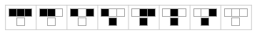
Although it seems unlikely a reader of this particular post has not heard of cellular automatons, for the sake of completeness, we give a brief introduction. In some ways, CAs are the simplest models we consider, despite the fact that they are capable of immense complexity. Cellular automaton obey simple, local update rules based on the neighborhood of the cell. In that way, they are the ideal playground for testing language model capabilities. The automaton itself evolves according to simple rules, yet under certain conditions can produce highly complex behavior. Below you can explore changing three parameters for the cellular automaton:
1) The rule number of the automaton, which tells each cell how to update based on the current cell state and its neighbors.
2) The width of the initial condition for the automaton.
3) The number of steps to compute; that is, the number of times the rule is applied.
Although the emergent behavior looks complicated, the process is completely deterministic and trivial to compute, provided you possess the patience to step through the computations. We predominantly use Rule 30 in our analysis.
In[]:=
RandomSeed[42];Manipulate[Column[{Style["Rule Description",{Alignment->Center}],RulePlot[CellularAutomaton[rule],ImageSize->Medium],ArrayPlot[CellularAutomaton[rule,RandomInteger[1,width],steps],ImageSize->{Medium,Automatic}]}],{width,5,50,1,Appearance->"Labeled"},{steps,1,50,5,Appearance->"Labeled"},{rule,30},Initialization:>(width=20;steps=4)]
Out[]=


The language models are given the full description of the rule, an initial configuration, and the number of steps to predict. Accuracy is measured averaged across all predicted cells.
Arithmetic Expressions
Arithmetic Expressions
Our next model is basic arithmetic expressions, using addition, subtraction, and multiplication. There’s a reasonably large literature on the performance of models on large scale computations (such as multi-digit multiplication) or numerical word problems. However, in keeping with the theme of fundamental, simple tasks, we analyze extremely simple expressions composed of operations on single digit numbers.
In order to generate these randomly, we create random binary trees in which the leaves of the tree are random values, the branch nodes are randomly selected operations. In this way, we can vary the expected difficult of the problems. However, to take this simple model one step further, we augment the way in which the binary trees are generated to create unbalanced trees. In effect, this means the computations are less parallelizable: errors computed on one part of the tree will invariably results in errors elsewhere.
An outline of the code is included below.
1
.To create a random expression, we create a recursive function which takes in the number of nodes, the branch node operations, and the bias associated with the tree. We create the binary tree by randomly splitting the remaining nodes into two groups, and recursing. As the bias term increases, the likelihood of using a lower splitting index increases, thus making the tree more right-balanced.
2
.Below we can visualize examples of these binary trees, toggling the number of nodes and the right-bias accordingly. Changing the toggle will generate a new tree each time.
In[]:=
Manipulate[Module[{randomTree},randomTree=RandomTreeExpression[nodes,{"Bias"->rightBias}];Column[{ExpressionDataPoint[randomTree],Show[randomTree,ImageSize->{Medium,Automatic}]}]],{{nodes,10},1,20,1,Appearance->"Labeled"},{{rightBias,1},1,10,1,Appearance->"Labeled"}]
Out[]=
The models are given the written form of the expression, and evaluated only on their final answers.
The models are given the written form of the expression, and evaluated only on their final answers.
Fool’s Chess
Fool’s Chess
By Fool’s Chess, we mean chess that need not follow any strategic pattern. The only restriction is that any sequence of moves must be valid according to the rules of chess. Want to move your knight back and forth six times while your opponent nears checkmate? Sure! Consider Fool’s Chess to be a single player game, where you may move the pieces around to your hearts content, within the constraints of the game.
In this task, the model is prompted to generate a sequence of moves which obey a set of restrictions. These restrictions all take the same form: The Nth capture should be an X capturing some piece, where X is either a pawn, a knight, or a bishop. We could conceivably come up with more complex restrictions, yet as we will see, the models will struggle even at this level.
Below you can generate random games, which will output the set of rules they abide by. When testing the models, we instead provide the sequence of rules, and ask for a sequence of moves.
In[]:=
ExplainChessGame[chessGame_]:=Module[{captureMoves,pieceNameMapping},captureMoves=Map[StringSplit[#,"x"][[1]]&,Select[chessGame["Moves"],StringContainsQ[#,"x"]&]];pieceNameMapping=Lookup[<|"Q"->"Queen","K"->"King","N"->"Knight","B"->"Bishop","R"->"Rook"|>,#,"Pawn"]&;capturePairs=MapIndexed[ToString[First[#2]]<>") "<>pieceNameMapping[#1]<>" captures\n"&,captureMoves];If[Length[capturePairs]===0,"No captures",StringJoin[capturePairs]]];Manipulate[chessGame=RandomChessGame[n,<|"White"->"Alice","Black"->"Bob"|>];Column[{ExplainChessGame[chessGame],ChessViewer[chessGame]}],{{n,20},10,40,2}]
Out[]=
The models are given a set of rules, and evaluated on (a) the validity of their move sequence and within those valid moves (b) their adherence to the supplied constraints.
Digression into Infrastructure
Digression into Infrastructure
Cellular Automaton
Cellular Automaton
What does the model see?
What does the model see?
Results
Results
Here we quickly load in the saved data using our helper function , group the data by the hyperparameters, and compute per bit accuracy across the results.
importTrialData
In[]:=
CellularAutomatonResults=importTrialData["/Users/Alex/Desktop/Wolfram Summer School/Project/Trials/FINAL_CA_PREDICTION.jsonl"];CellularAutomatonPlotData=GroupBy[CellularAutomatonResults,{#ModelName&,#AdditionalParameters["Steps"]&,#AdditionalParameters["Width"]&},Function[trialSet,(*Wetakemeanstwice(perelementintheautomaton,thenpertrialgroup),butsincethesizeofeachautomatonresultshouldbethesame,thusitisequivalenttodeterminingthebitwisemeanacrossallpredictions.*)Mean[Map[If[Head[#ExtractedLLMOutput]===List,(*Return0correctiftheformatisincorrect*)Mean[Map[Boole@*SameQ@@#&,(*Ifoneresultisbiggerthantheother,usetheminimumlength.*)minThread[{#ExpectedOutput,#ExtractedLLMOutput}]]],0]&,trialSet]]*100]];
We plot the data with reference lines around 40%, 50%, and 60%. These lines are arbitrary, but helpful to contextualize the accuracy rates.
We add o1-mini for reference, although due to cost restrictions the total number of trials is much lower. There are a few trends worth pointing out.
Firstly, the width of the automaton has little bearing on the overall accuracy. Given the locality of the calculations, this may be expected a priori, yet models do often get confused with additional unnecessary information. At least at the lengths being considered, the width of the automaton seems to have little bearing on the overall accuracy. Secondly, one forward pass seems insufficient even to perform even a single application of the rule. This is quite surprising, as each outputted token could get a single forward pass all to itself, meaning the model need only determine which of the 8 rules to apply given the proceeding context. With this in mind, it’s unsurprising that the subsequent steps become indistinguishable from random guessing.
Despite being a rather straightforward inference, it seems the models haven’t fully generalized the ability to follow such a simple set of rules. So we now move to something which is almost certainly in the training data, where the computation cannot be parallelized across different forward passes: arithmetic!
Arithmetic Expressions
Arithmetic Expressions
Results
Results
Again, we can load in the results with our helper function, and then group by the hyperparameters.
The result, at least to me, are somewhat surprising. Firstly, there seem to be no significant trends differentiating parallel and sequential computation. The model seems to be, in a highly anthropomorphized sense, doing all the computation at once. Moreover, one would expect that larger models have the capacity to perform significantly more computation, are therefor should perform at least notably better for a problem of the same complexity. But in fact, we see for small equations the smallest model performs notably better, and they do so especially in cases where the computation can be parallelized. The rate of decay is modestly slower as the expression size increases as well, indicating the smaller model is indeed superior in this highly limited domain of single digit arithmetic.
This might be the most surprising finding thus far, although we still have something in store. We discuss some potential explanations for this phenomenon in the conclusion, but needless to say it’s perplexing. For reference, here is the performance for each of the models on the most balanced subset of trees.
This might be the most surprising finding thus far, although we still have something in store. We discuss some potential explanations for this phenomenon in the conclusion, but needless to say it’s perplexing. For reference, here is the performance for each of the models on the most balanced subset of trees.
Fool’s Chess
Fool’s Chess
What does the model see?
What does the model see?
Our goal is to generate a set of random constraints of varying sizes, and pass this information to the model so it may generate a sequence of chess moves. Recall the restrictions are of the simple form “The Nth capture should be X capturing a piece”, where we exclude rooks, queens, and kinds from the set of possible values for X.
Again, we generate the results by supplying a the prompt, specifying the number of conditions (rules) for the LLM to adhere to, and using our nicely defined built-ins.
Again, we generate the results by supplying a the prompt, specifying the number of conditions (rules) for the LLM to adhere to, and using our nicely defined built-ins.
Results
Results
By now you know the drill. Helper function for the data, group by, and pretty plot!
The results here are some of the most surprising (I think I said that before, but now I really mean it). In isolation, I’m not completely surprised at the models’ tenancy to make up nonsense, as indicated by the plateauing valid moves with ever-increasing total moves (valid moves, in this case, refer to legal moves, regardless of the correctness according to our constraints). This also explains why the percentages (left most graph) look monotonically(ish) decreasing, since the likelihood of even having 8 valid captures at all seems to diminish as the total number of moves increases. However, most surprising about this graph is that o1-mini holds no edge over the zero-shot, no chain-of-thought frontier model, and barely any over its inferior companions! Given the ample availability of internet data about chess, I find it rather surprising that the models are so embarrassingly poor at constructing games under these rather loose conditions! As with before, more on this in the conclusion.
Concluding Remarks
Concluding Remarks
Initially, I wanted to test how basic networks are able to predict simple computational phenomenon, like some of the tasks described above. Quickly I found that indeed they predicted them quite poorly, poorly enough that a notable amount of infrastructure may be required to appropriately run large scale variations in model architecture and size. The natural follow up, then, was to build on the millions (billions?) of dollars of infrastructure already invested by frontier AI companies. What we find is that these models not only display clear deficiencies in reasoning, but more general inconsistency in returns to scale, both in pre-training and inference: bigger models don’t always perform better on simple tasks, and occasionally perform worse, contrary to theoretical expectations.
The case of cellular automaton is the most clear cut. Despite describing exactly the update rule to be follow... sorry I’m going to interrupt myself. I need to spell this out in excruciating detail: just a few lines before giving the initial state, the model very explicitly has the rules written for it as “001->1”, “101->0”, etc. And yet, upon generating the next token to complete just a single step of the automaton, it cannot consistently follow this rule one token at a time. That means it knows it’s about to predict another token, it can read off precisely the three tokens in the neighborhood, and can read off precisely the mapping all in the same paragraph, and yet it still fails miserably. The hope of accomplishing even more computational steps is lost by this point without chain-of-thought reasoning, but I read these results as quite damning for these frontier models.
So perhaps it’s unfair we follow up with an even more difficult task to follow up. Arithmetic, we all know, is not at which something models excel. Yet despite rapidly diminishing accuracy as the expression proceeds (which was expected), we still find a few interesting kernels. Firstly, the models don’t seem to be utilizing parallelized computation, or at least if they are, it doesn’t seem to be helping very much. The results seemingly never vary depending on how sequential the expressions are, with the notable exception of our tiny friend gpt-4.1-nano, who outperforms her older siblings on smaller tasks and seems to take advantage of the parallelizable.
There are a few reasons this might be: firstly, the larger models might have been fine-tuned further on general dataset, due to their generally-more-impressive capabilities. This could have the affect of crushing their arithmetic capabilities, which aren’t critical to their function anyway, whereas perhaps the smaller models get a lighter touch. Alternatively, the larger models may be “over-thinking” the problem, through some internal hallucinations where further computation isn’t necessary. Thirdly, and most speculatively, perhaps the kinds of tasks real consumers request for the smallest models somehow rely most heavily on raw computation, like API calls into a spreadsheet or market analysis. Frankly, these all seem quite dubious to me, and I remain unconvinced and surprising!
Finally, we have chess, the game of Kings! Anecdotally, these experiments have also been tried with all of the latest frontier reasoning models, and it’s safe to say that no model has internalized chess. Not only are the moves themselves never in accordance with the suggestions, but they quickly devolve into nonsense, indicating something like a complete lack of spatial reasoning. It’s worth noting explicitly: if you know the rules of chess, you should try a few of these problems on your own. See if you can create a game with a pawn capture, a knight capture, and then a bishop capture, where there are no other restrictions on the strategic advantage of your moves. It is, for someone who can see the board, trivially easy, much easier than it sounds!
With each of these experiments, we really only have a pointer towards a class of interesting problems: the simplest problem, which defeats all the models; a difficult problem briefly dominated by the smallest model; and an open-ended problem which stumps even the reasoners. There are many directions to take these results, both separately and together, but together these results leave me feeling a bit more optimistic about my job prospects in the coming years :)
Acknowledgments
Acknowledgments
I want to thank Christopher Wolfram and Daniel Sanchez, my mentors during the Wolfram Summer School. Christopher’s deep knowledge of the Wolfram Language was instrumental in accelerating my WL learning curve, and his conceptual guidance helped ensure the scope was both interesting and achievable. Daniel provided invaluable resources from the Wolfram archive and connections to experts, as well as his valued guidance on this project’s topic matter in the middle and early stages.
I want to also thank Stephen for his expertise during the initial brainstorming stages of the project, and of course, Stephanie for flawless managing to bullseye every moving target for three weeks straight.
I want to also thank Stephen for his expertise during the initial brainstorming stages of the project, and of course, Stephanie for flawless managing to bullseye every moving target for three weeks straight.
References
References
1
.S. Wolfram (2002), A New Kind of Science. Wolfram Media.
Cite This Notebook
Cite This Notebook
“Limits of Language Model Computation”
by Alex Fogelson
Wolfram Community, July 9th, 2025
https://www.wolframcloud.com/env/fogelson/Published/Limits%20of%20Language%20Model%20Computation.nb
by Alex Fogelson
Wolfram Community, July 9th, 2025
https://www.wolframcloud.com/env/fogelson/Published/Limits%20of%20Language%20Model%20Computation.nb