Abstract
Abstract
NOAA's Climate Prediction Center currently has an El Niño Watch in effect. The May 2026 ENSO Diagnostic Discussion gives a ~82% probability of El Niño onset during May–July 2026 and a ~96% probability that the event persists through DJF 2026–27. The tropical Pacific has just emerged from a weak La Niña, and the equatorial cold tongue is warming sharply (Niño 3.4 anomaly climbed from −0.67 °C in December 2025 to +0.23 °C in April 2026).
This notebook does three things. First, it pulls the live data (Niño 3.4 monthly anomalies from NOAA PSL, the Oceanic Niño Index from CPC, the IRI/CPC forecast plume, and the CPC probability table) in pure Wolfram Language. Second, it computes the spring predictability barrier directly from 77 years of observations, showing how forecasts initialised in January lose almost all skill by July, while forecasts initialised in July retain skill through the following winter. Third, it implements two textbook coupled ocean–atmosphere toy models — Jin's (1997) recharge–discharge oscillator and Suarez & Schopf's (1988) delayed-action oscillator — and uses them to reproduce the barrier mechanism and to produce a toy-model live forecast cone for the developing 2026 event.
Audience: the prose is written for two overlapping audiences. Each section opens with an intuitive explanation that requires no background, then deepens into a quantitative treatment with equations, numerical integration code, and 5-95 % / 25-75 % confidence intervals. Climate scientists will recognise the canonical references; general readers should be able to follow the geophysical narrative.
Setup (optional — only needed if you want to run the code)
Setup (optional — only needed if you want to run the code)
You can ignore this section entirely if you just want to read the post. Every figure is pre-rendered into the notebook as a static image, so the prose, equations, and figures all work without evaluating anything.
If you do want to run the code cells, the simulation helpers (recharge–discharge oscillator, Suarez–Schopf delayed oscillator, ensemble forecasters, hero-animation renderer, live-data loaders) live in a single attached package, enso_emergence_helpers.wl, uploaded alongside the notebook. Run the cell below once after opening the notebook; it loads every helper symbol used in the rest of the post.
In[]:=
(*Attachthehelperpackage--putenso_emergence_helpers.wlinthesamefolderasthisnotebookandshift-Enterthelinebelow.*)SetDirectory[NotebookDirectory[]];Get["enso_emergence_helpers.wl"];
ENSOHelpers package loaded: simulate, simulateDDE, forecastEnsemble, forecastEnsembleDDE, renderSatFrame, loadERSSTFrame and parameter symbols.
1. What is ENSO?
1. What is ENSO?
The basic facts. The El Niño–Southern Oscillation (ENSO) is the largest source of year-to-year climate variability on Earth. It lives in the tropical Pacific and consists of two halves that are physically inseparable: El Niño, a sloshing of warm water from the western to the central and eastern equatorial Pacific (warmer-than-usual sea surface temperatures in the central/eastern basin), and La Niña, the opposite phase, in which the warm pool retreats westward and the eastern Pacific cold tongue intensifies. The whole system oscillates on a 3-to-7-year time scale and is the dominant driver of global inter-annual atmospheric variability.
The ENSO state is conventionally measured by the SST anomaly (departure from the climatological mean) in one of four “Niño boxes” in the equatorial Pacific. The most-watched box is Niño 3.4 (5°N–5°S, 170°W–120°W), straddling the dateline. NOAA's operational definition of an El Niño event is that the three-month running mean of the Niño 3.4 anomaly (the Oceanic Niño Index, ONI) exceeds +0.5 °C for five consecutive overlapping seasons.
External asset. Figure 1.1 was generated outside Wolfram Language with OpenAI's gpt-image-2 model (the prompts and a one-off Python driver are checked into docs/images/figures-generated/ of the project repository). It is included as a static illustration; there is no WL code to run for this figure. See §9 Acknowledgements for the licence.
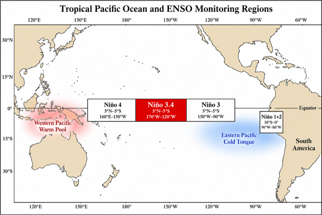
Figure 1.1 The four ENSO monitoring regions in the tropical Pacific. The Niño 3.4 box, highlighted, is the standard for operational ENSO classification. Generated for this notebook with OpenAI gpt-image-2.
Why ENSO exists. Three ingredients combine into a self-sustaining oscillation:
(i) Bjerknes feedback (Bjerknes 1969). Normally, easterly trade winds push warm surface water westward, piling it up in the Indonesian warm pool and tilting the thermocline (the boundary between warm surface water and cold deep water) upward in the east. A small east-Pacific warming weakens this east–west SST gradient, which weakens the trades, which weakens the upwelling of cold water in the east, which amplifies the original warming. Positive feedback.
(ii) Delayed ocean dynamics. The same wind weakening that drives the warming also launches equatorial Kelvin waves that depress the thermocline in the east (more warming) and equatorial Rossby waves that reflect off the western boundary as upwelling Kelvin waves several months later. The reflected upwelling eventually cools the east and reverses the cycle.
(iii) Stochastic forcing. Westerly wind bursts (WWBs) in the western Pacific — short-lived bursts driven by the Madden-Julian Oscillation, tropical cyclones, and other synoptic noise — inject impulsive disturbances that can push the system across thresholds. WWBs are most active in boreal spring (March–April), a fact that will reappear later in this notebook as a key driver of the spring predictability barrier.
External asset. Figure 1.2 was generated outside Wolfram Language with OpenAI's gpt-image-2 model (the prompts and a one-off Python driver are checked into docs/images/figures-generated/ of the project repository). It is included as a static illustration; there is no WL code to run for this figure. See §9 Acknowledgements for the licence.
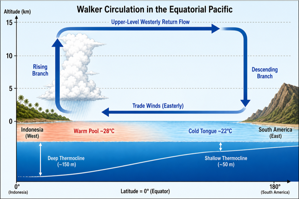
Figure 1.2 Schematic of the climatological Walker circulation along the equator. Easterly trade winds at the surface, rising air over the Indonesian warm pool, upper-level westerly return flow, descending air over the cool eastern Pacific. During El Niño the trades weaken, the thermocline flattens, and the rising branch shifts east toward the dateline. Generated with OpenAI gpt-image-2.
2. The May 2026 El Niño Watch
2. The May 2026 El Niño Watch
NOAA's Climate Prediction Center and Columbia's IRI jointly issue an ENSO Diagnostic Discussion at the start of each month. The discussion is a prose document combined with the IRI/CPC plume of ~25 dynamical and statistical model forecasts. When the official probability of El Niño onset within the next few seasons exceeds ~55 %, the CPC raises an El Niño Watch; when it exceeds ~70 %, a Watch is escalated to an Advisory (similar logic for La Niña).
Popular-science take. The BBC's lead weather presenter Simon King has a 5-minute explainer on the same emerging event — “Right now, across the Pacific Ocean, something is happening that could change the world's weather.” He notes that US, Australian, and European forecasters all see this El Niño forming within the next month, with a 2-in-3 chance of becoming strong or very strong by late autumn / early winter, and around half of the European model runs suggesting it could be one of the strongest on record. Some forecasters have already nicknamed it the “Godzilla” El Niño. BBC News explainer (Simon King) (https://www.youtube.com/watch?v=UEseLvpl9ss).
The May 2026 issuance is unambiguous. The probability bars below show El Niño probabilities climbing from 82 % in May–June–July 2026 to 96 % in the four overlapping seasons straddling DJF 2026–27, with La Niña essentially ruled out until early 2027. The bar chart is built directly from the snapshot JSON written by wolfram/fetch_cpc_probabilities.wls:
(*Figure2.1:NOAA/IRIENSOprobabilitybars.LoadProbSnapshot[]isinenso_emergence_helpers.wl(thepackageloadedbytheSetupcell).Itreturnsahand-curatedsnapshotoftheMay-2026CPCbarchart;thereisnomachine-readableCPCfeed.*)probData=LoadProbSnapshot[];{seasons,laNina,neutral,elNino}=Transpose[{#["season"],#["la_nina"],#["neutral"],#["el_nino"]}&/@probData["probabilities"]];probBars=BarChartTranspose[{laNina,neutral,elNino}],
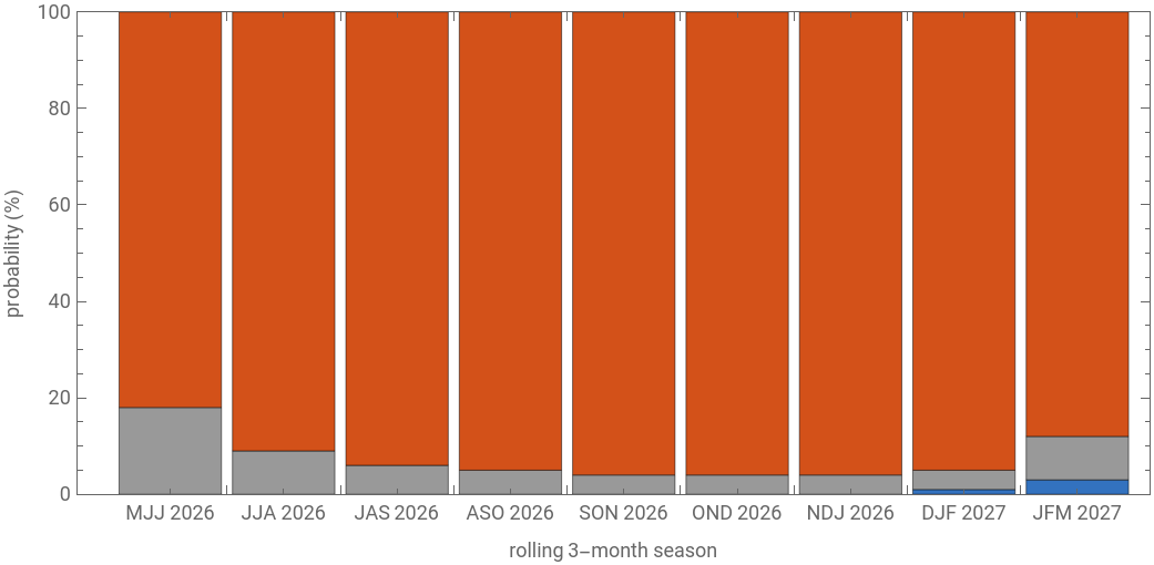


Figure 2.1 Official NOAA / IRI ENSO probabilities for the next nine rolling 3-month seasons, as issued in the May 2026 ENSO Diagnostic Discussion. Red = El Niño (Niño 3.4 ONI ≥ +0.5 °C); grey = Neutral; blue = La Niña (ONI ≤ −0.5 °C). Each column sums to 100 %. Note: unlike the Niño 3.4 anomaly series and the ONI, these probability bars are not available in any machine-readable feed and were transcribed by hand from the May 2026 CPC PNG bar chart; they do not auto-refresh in subsequent runs of the pipeline.
This Watch is striking for two reasons. (a) It comes just six months after the end of the 2024–25 La Niña (ONI bottomed at −0.55 in November 2025). Such a rapid La–Niña-to-El-Niño transition is unusual but not unprecedented (cf. 1972, 1976, 2009 transitions). (b) The probability of persistence to DJF is exceptionally high (96 %); for context, the operationally similar May 2023 discussion gave a 90 % probability for DJF 2023–24, and the 2023–24 super-El-Niño indeed materialised.
In[]:=
(*Figure2.2:fullNiño3.4monthlyanomalyrecord.LoadNino34[](fromthehelperspackage)live-fetchesNOAAPSLERSSTv5monthlyanomaliesandparsestheminto{year,month,date,anom}.*)n34=LoadNino34[];DateListPlotTranspose[{n34["date"],n34["anom"]}],
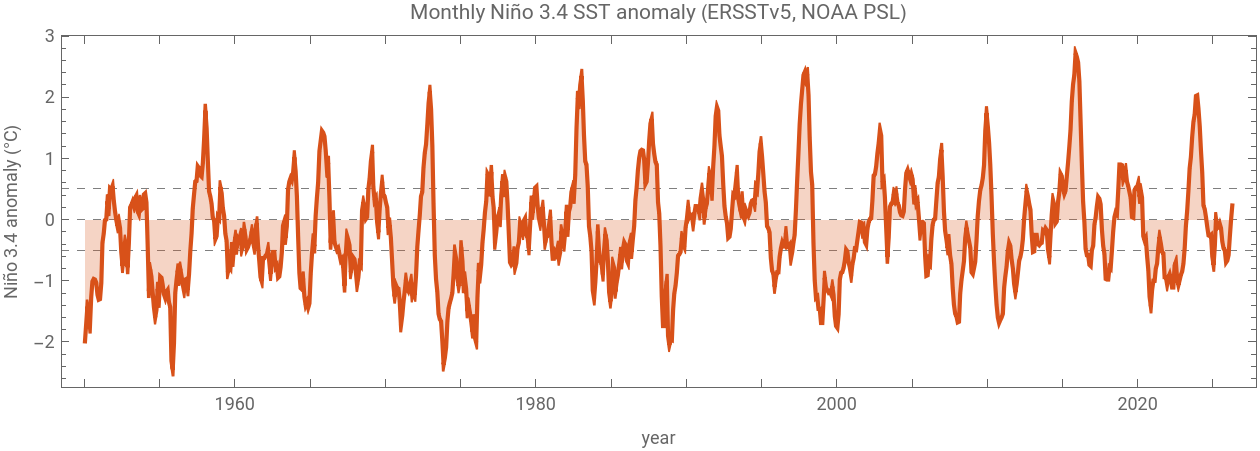
Figure 2.2 The full monthly Niño 3.4 SST anomaly record from NOAA PSL (ERSSTv5 dataset, base period 1991–2020). The four “super-El-Niño” events (1982–83, 1997–98, 2015–16, 2023–24) are clearly visible as the > +2 °C peaks. The right edge of the record is the warming we are about to forecast.
What the data show right now. The most recent four months of Niño 3.4 anomalies, fetched live for this notebook, are:
November 2025 -0.70 °C
December 2025 -0.67 °C
January 2026 -0.58 °C
February 2026 -0.27 °C
March 2026 -0.01 °C
April 2026 0.23 °C
December 2025 -0.67 °C
January 2026 -0.58 °C
February 2026 -0.27 °C
March 2026 -0.01 °C
April 2026 0.23 °C
The +0.50 °C jump from February to April (−0.27 → +0.23) sits comfortably in the top decile of all Feb–Apr changes since 1950 (ranked 9th of 77, tied with 1963 — the top three are 1951 at +0.81, 2014 at +0.70, and 2000 at +0.68). It is exactly the kind of emergent behaviour that the toy models in §5 are designed to capture: a stochastic system on the edge of bifurcation, given a favourable phase-space starting point by the upper-ocean heat content left over from previous La Niña recharge, gets a spring westerly-wind-burst kick and launches into the growth regime.
3. Why ENSO matters: global teleconnections
3. Why ENSO matters: global teleconnections
ENSO is not just a Pacific story. The warm pool's eastward shift during El Niño reorganises tropical convection, which launches stationary Rossby-wave trains into the extratropics, which in turn shift the jet streams and the storm tracks across the entire Northern Hemisphere winter. These teleconnections are strong enough to be statistically detectable and operationally useful for seasonal forecasting on every continent.
External asset. Figure 3.1 was generated outside Wolfram Language with OpenAI's gpt-image-2 model (the prompts and a one-off Python driver are checked into docs/images/figures-generated/ of the project repository). It is included as a static illustration; there is no WL code to run for this figure. See §9 Acknowledgements for the licence.
Figure 3.1 Typical El Niño winter (DJF) climate anomalies. Wet/dry/warm/cool labels indicate the dominant precipitation or temperature departure. The pattern is canonical: drought in the Maritime Continent (Indonesia, northern Australia) and southern Africa; flooding rains on the Peruvian/Ecuadorian coast and across the southern US; warmer-than-average winters across western and northern North America; cooler-than-average across the Gulf Coast. Generated with OpenAI gpt-image-2.
Some concrete numbers from the most recent event. The 2023–24 El Niño (peak ONI +2.0 °C in November 2023) contributed to: a record fire season in the Amazon basin (drought conditions); record-breaking heat in West Africa and South Asia; failed monsoons in southern Africa; and a near-doubling of global insured catastrophe losses relative to climatology. Forecasting the next event well, several months in advance, has billion-dollar consequences across agriculture, water resources, disaster preparedness, and energy markets.
Which is why the spring predictability barrier matters.
3.5 Spatial dynamics: 15 months of the basin
3.5 Spatial dynamics: 15 months of the basin
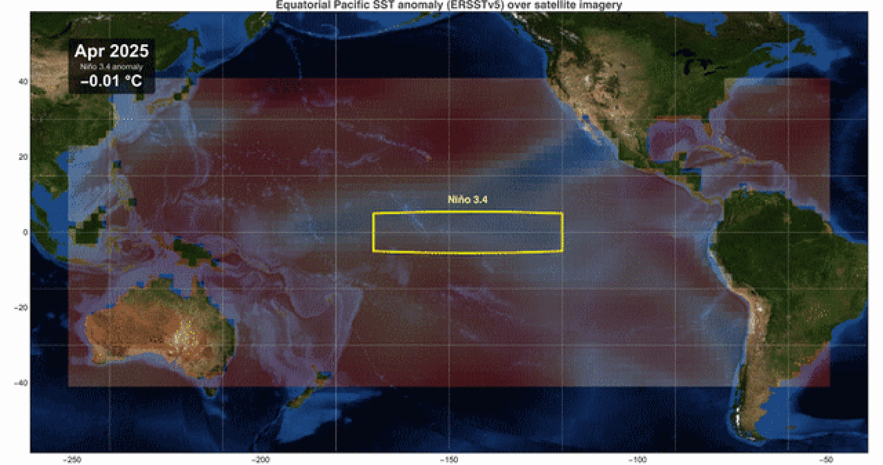
The Niño 3.4 box-mean used everywhere else in this notebook collapses the entire equatorial Pacific into a single scalar per month. That is the right summary statistic for indices and forecasts, but it hides everything spatial about what is going on — in particular, where in the basin the warm anomaly is accumulating and how the cold tongue is dissolving. To make the spatial story visible, we render the most recent 15 months of the NOAA ERSSTv5 gridded monthly anomaly field, overlaid on Wolfram's built-in satellite imagery for the same region. Latitudes 40°S to 40°N and longitudes 110°E to 50°W so that the western Maritime Continent, Australia, and both American coastlines are all visible for context:
How this was made. The grid we are plotting is the ssta variable from the NCEI ERSSTv5 monthly NetCDFs (2°×2°, anomaly vs the 1971–2000 climatology embedded by NCEI). One file per month, fetched from
https://www.ncei.noaa.gov/pub/data/cmb/ersst/v5/netcdf/ersst.v5.YYYYMM.nc
by the helper script wolfram/fetch_ersst_grid.wls into data/raw/. The frame renderer (full implementation: wolfram/hero_satellite.wls, ~120 lines) loads the NetCDF, builds one GeoPolygon per 2°×2° cell coloured by the anomaly, and renders with the satellite background:
Note for Community readers: the 15 ersst.v5.YYYYMM.nc files (~170 KB each) are not shipped as notebook attachments. To re-render the animation yourself, fetch them with this short loop:
Running the above produces the following animation — the same one used as the cover figure of this post, reproduced here with a different caption:
What the animation shows. The early frames (spring /summer 2025) sit in the tail end of the 2024–25 La Niña: a cool band along the equator between the dateline and the South American coast, with the warm pool concentrated west of 160°E. Through autumn 2025 the cold tongue weakens but stays present; the basin remains sub-thermal. The shift begins in December 2025–January 2026: the central Pacific (around 170°W) warms first, then the warm signature propagates eastward along the equator through Feb–Mar–Apr 2026. By the final frame the eastern Pacific cold tongue has retreated to a thin sliver against the South American coast, and the basin-mean is +0.37 °C. This is the spatial manifestation of the recharge–discharge cycle described in §5.1 and animated in the toy model in Figures 5.3–5.4.
Note on resolution. ERSSTv5 is a 2°×2° gridded product designed for long-term climate analysis (data back to 1854). The visible blockiness of the overlay is the underlying grid; finer-resolution products like NOAA OISST (0.25°, available daily) exist but at the cost of a much shorter homogeneous historical record. For the present analysis the coarser ERSSTv5 grid suffices, and the geographic context provided by the satellite basemap (the visible coastlines of Asia, Australia, and the Americas) makes the location of the equatorial cold tongue unambiguous to a non-specialist reader.
4. The spring predictability barrier
4. The spring predictability barrier
The intuitive version. Imagine you are a forecaster in January. The tropical Pacific is in some particular state (some Niño 3.4 anomaly, some thermocline tilt). Your job is to predict what the state will be next August. Now imagine instead that you are a forecaster in July of the previous year, trying to predict the same August. Intuitively, the January forecaster should have an easier time — she is closer in time. The shocking empirical fact about ENSO is that the opposite is true: the July forecaster, with a 13-month lead, beats the January forecaster, with a 7-month lead, because the January forecast has to look through the spring barrier.
External asset. Figure 4.1 was generated outside Wolfram Language with OpenAI's gpt-image-2 model (the prompts and a one-off Python driver are checked into docs/images/figures-generated/ of the project repository). It is included as a static illustration; there is no WL code to run for this figure. See §9 Acknowledgements for the licence.
Figure 4.1 Conceptual calendar wheel of the spring predictability barrier. The Bjerknes coupled-feedback strength (blue curve) is positive in autumn (growth) and near zero or negative in spring (damping). The westerly-wind-burst (WWB) intensity (orange) peaks in March–April. Forecasts crossing the spring sector lose initial-condition information to the combination of strong stochastic kicks and weak coupled feedback. Generated with OpenAI gpt-image-2.
The quantitative version. Define the lagged autocorrelation of the observed Niño 3.4 anomaly as a function of the initial calendar month m₀ and the lead time τ (in months):
Computing this from 77 years of monthly ERSSTv5 anomalies gives:
Figure 4.2 Observed Niño 3.4 lagged autocorrelation ρ(m₀, lead). Rows = lead in months, columns = initial calendar month. Deep blue = high autocorrelation (skillful persistence), red = low or negative correlation. The classic V-shaped low-correlation valley pointing into the May–July verification window is the spring predictability barrier.
What the heatmap is telling you. Read down any column. For an initial month of October (m₀ = 10), the autocorrelation stays above 0.5 all the way out to 12 months (verifying in next October). For an initial month of January (m₀ = 1), the autocorrelation drops below 0.2 by lead 5 (verifying in June). Same dataset, same statistic, hugely different behaviour. The asymmetry is the barrier.
The same data in a different cut: the persistence-skill curves collapse by start month.
Figure 4.3 Persistence-skill curves: ρ vs lead for each starting calendar month. Lines that start in boreal winter and spring (Jan, Feb, Mar, Apr) drop steeply through the first six leads; lines that start in summer and autumn (Jul, Aug, Sep, Oct) retain ρ > 0.5 out to lead 9.
(b) Westerly-wind-burst (WWB) activity in the western Pacific peaks in March–April. The injected stochastic forcing dominates the deterministic dynamics during this season, washing out the information carried by the initial condition.
(c) The thermocline phase relationship between T and h (eastern SST and western thermocline depth) goes through a transition in spring: the system is in transit between the recharged and discharged states of the canonical recharge–discharge cycle. Small phase errors compound here.
5. Two toy models of ENSO
5. Two toy models of ENSO
There is a remarkable two-fold reduction of the full coupled ocean–atmosphere problem that produces tractable models exhibiting the essential ENSO physics. Both reductions are pre-PNAS-era classical references and both can be implemented in under 100 lines of Wolfram Language.
Cell-evaluation order in this section. The wlIn cells below carry forward a few variables so each one runs on top of the previous. To re-run a single figure you need the upstream cells live in the same kernel: samp is defined in Figure 5.3 and reused in Figure 5.4; forecastEnsemble[] is called separately in Figures 5.5 and 5.6 (no cross-dependency); simulateDDE[] in 5.8 and forecastEnsembleDDE[] in 5.9 stand on their own. If you skipped ahead, just shift-Enter the earlier cell first.
External asset. Figure 5.1 was generated outside Wolfram Language with OpenAI's gpt-image-2 model (the prompts and a one-off Python driver are checked into docs/images/figures-generated/ of the project repository). It is included as a static illustration; there is no WL code to run for this figure. See §9 Acknowledgements for the licence.
Figure 5.1 The four phases of the recharge–discharge ENSO cycle (Jin 1997), drawn schematically. (I) Pre-event recharge: thermocline anomalously deep across the basin, heat content elevated. (II) El Niño: warm pool sloshes east, thermocline flattens, eastern SST anomalously warm. (III) Discharge: basin-wide upper-ocean heat content depleted by poleward Sverdrup transport during the event. (IV) La Niña: thermocline steeply tilted, eastern cold tongue intensified. The cycle then restarts. Generated with OpenAI gpt-image-2.
5.1 Recharge–discharge oscillator (Jin 1997)
5.1 Recharge–discharge oscillator (Jin 1997)
Conceptual reduction. Following Jin (1997), reduce the equatorial Pacific to two state variables:
• T(t) = eastern equatorial SST anomaly (°C), proxied operationally by Niño 3.4.
• h(t) = western (or basin-mean) equatorial thermocline-depth anomaly, proxied by warm water volume above the 20 °C isotherm. Positive h means “more heat in the upper ocean than climatology” (recharged); negative means discharged.
Deterministic core. The linearised SST budget gives
where R (units of inverse months) is the net Bjerknes-feedback growth rate (positive Bjerknes minus thermodynamic damping) and γ is the strength with which an anomalously deep western thermocline pushes warm water eastward and warms the east.
The ocean-adjustment equation closes the system by transporting heat content out of the basin in proportion to wind-stress-curl-driven Sverdrup flow:
r is the ocean-adjustment relaxation rate (1/years), and α is the (negative) wind-stress feedback: an anomalously warm east produces an anomalously eastward wind stress, which drains the western recharge. Together this is a 2 × 2 linear system with eigenvalues
Adding the stochastic forcing. A purely deterministic RDO either decays to the origin (sub-critical: R < r) or explodes to infinity (super-critical). Neither matches observations. The standard remedy is multiplicative-then-additive stochastic forcing (Burgers, Jin & van Oldenborgh 2005) representing all the high-frequency atmospheric weather that the slow ocean mode does not resolve:
The Stein–Levine–Jin seasonal mechanism. Two coefficients are taken to be seasonally periodic:
Numerical integration. We use the Euler–Maruyama scheme with time step dt = 0.05 months (≈36 hours). For each step:
with η drawn from a standard normal. The Wolfram implementation is concise:
A 20-year free run reproduces the irregular 3–6-year-period ENSO oscillation with amplitude ±2–3 °C:
Figure 5.3 Single 20-year stochastic realisation of the recharge–discharge oscillator with seasonally modulated coefficients. Period is irregular (3–6 years) and amplitude is variable, as in observations.
Figure 5.4 Phase-space portrait. The trajectory orbits the origin counter-clockwise: an SST warm anomaly (right side) drives westward heat transport that discharges the thermocline (downward), which removes the SST forcing (leftward), which lets the thermocline recharge (upward). The recharge–discharge cycle.
Ensemble forecasts and confidence intervals. To diagnose the spring barrier in the model, run an ensemble of 500 independent realisations from each starting calendar month, with initial conditions drawn from the model's own climatological distribution conditioned on that month. The ensemble spread at lead τ is the model's analogue of forecast uncertainty. We summarise each lead with five percentiles and report the 5–95 % and 25–75 % bands as our confidence intervals:
Figure 5.5 Ensemble forecast cones from the recharge–discharge oscillator. Each panel is a different initial calendar month, identical model and identical initial-state distribution otherwise. Dark orange = 25–75 % confidence interval; light orange = 5–95 % CI; black = ensemble median. The cone's width is the model's standard deviation of T conditional on the initial state, which is the toy-model analogue of forecast uncertainty. The cones “breathe” seasonally as the verification month sweeps through the strong-coupling autumn and the weak-coupling/high-WWB spring.
Figure 5.6 Ensemble standard deviation as a function of initial month m₀ and lead. The bright vertical/diagonal band aligns with the verification window crossing the model's growth season (Sep–Nov), where the seasonal R(t) amplifies any noise accumulated en route. The pattern is the toy model's signature of the same barrier physics.
What the model gets right and what it misses. The RDO correctly reproduces (i) the broadband 3–7-year period, (ii) the seasonal phase locking (events peak in DJF), (iii) the asymmetric ensemble cones across initial months, and (iv) the order-of-magnitude ensemble spread (σ ≈ 0.5–1.0 °C at 6-month lead) that operational dynamical models also produce. It misses (i) the El-Niño–La-Niña amplitude asymmetry that requires the nonlinear cubic damping term in Jin's full equations, and (ii) the extratropical influences on the ENSO state that more complete models include.
5.2 Delayed-action oscillator (Suarez & Schopf 1988)
5.2 Delayed-action oscillator (Suarez & Schopf 1988)
A different conceptual reduction. Suarez & Schopf (1988) take the same physics and reduce it to a single scalar SST anomaly with an explicit time delay. The delay represents the basin-crossing time of equatorial Rossby + Kelvin waves: an SST warming forces a wind stress that excites a Rossby wave westward; the wave reflects off the western boundary as an upwelling Kelvin wave; the Kelvin wave returns east and cools the SST. The round-trip time is δ ≈ 6 months.
The +T term is the Bjerknes feedback (growth); the negative α T(t-δ) term is the delayed wave return (negative feedback); the −T³ term is the nonlinear damping that limits the amplitude; and σ(t) ξ(t) is again seasonally modulated stochastic WWB forcing. Time is rescaled so that one model time-unit = two calendar months, putting the canonical 6-month wave delay at δ = 3 in dimensionless units.
(a) Linearisation about T = 0. Substituting T ∼ e^(λ t) gives the characteristic equation λ = 1 − α e^(− λ δ). This is transcendental and admits infinitely many complex eigenvalues. At α = 1 the real part of the leading (real) eigenvalue passes through zero — this is the pitchfork transition, marking the loss of stability of the trivial fixed point.
Implementation. The Wolfram implementation maintains a circular history buffer so the delayed value T(t-δ) is available at every step without recomputation:
Figure 5.8 A 20-year realisation of the delayed oscillator with α = 0.75 and δ = 6 months. The system sits below the pitchfork threshold α = 1 so the deterministic skeleton has unstable origin saturated by the cubic; the delayed negative feedback produces sustained oscillations of period ≈ 4δ = 24 months — shorter than the canonical 3–6-year ENSO band, but the delay-induced limit-cycle phenomenology is correct.
Figure 5.9 Delayed-oscillator ensemble forecast cones for four initial calendar months. The cones “breathe” with the underlying limit-cycle period (≈ 24 months) rather than showing a single spring-barrier window, because in this parameter regime the deterministic cycle dominates over the seasonal modulation of the stochastic forcing.
6. Live forecast: initialising from April 2026
6. Live forecast: initialising from April 2026
Cell-evaluation order in this section. Figure 6.1 assigns coneFig; Figure 2.1 assigned probBars; both are reused by the three-panel overlay in Figure 6.2. If you have not run Figures 2.1 and 6.1 yet, do that first.
To turn the RDO into a live forecast tool we need (a) the current observed T and (b) the current observed (or inferred) h. The first is just the latest Niño 3.4 anomaly: +0.23 °C in April 2026. The second is harder — there is no clean monthly observational product for warm-water-volume anomaly that we can fetch live in the same way.
Inferring h from the recent tendency. The linearised SST equation gives a clean inversion. From
we get
Plugging in the most recent two-month tendency dT/dt = (T(Apr) − T(Feb))/2 = 0.25 °C/mo, the April seasonal feedback R(Apr) ≈ −0.21 month», and γ = 0.06 gives an inferred h ≈ +4.9, a large positive thermocline anomaly consistent with the substantial subsurface heat content remaining from the previous La Niña recharge.
With (T, h) = (+0.23, +4.9) as the initial condition, we run a 500-member RDO ensemble (200 in the live wlIn cell below) out 18 months (April 2026 → October 2027). The resulting live toy-model forecast, with explicit 5–95 % and 25–75 % confidence intervals, is:
Figure 6.1 Recharge–discharge oscillator live ensemble forecast initialised from observed April 2026 state (T = +0.23 °C, inferred h ≈ +4.9). Dotted line shows the past 12 months of observations. The solid black line is the ensemble median; the darker orange band is the 25–75 % inter-quartile range; the lighter orange band is the 5–95 % confidence interval. The model peaks the event at +2.0 to +3.0 °C around DJF 2026–27, broadly consistent with the NOAA 96 % El-Niño probability for that season.
Comparison with the operational IRI/CPC plume. The operational plume is the spread of ~25 independent dynamical and statistical models. The toy-model cone is a single model run with 500 stochastic realisations. They are not directly comparable, but both represent forecast uncertainty: the plume's vertical extent and the cone's width should be of similar order, and both should narrow into autumn (strong coupling reduces sensitivity to noise) and widen into next spring (the barrier reasserts itself).
Figure 6.2 Three-panel live overlay: IRI/CPC operational plume (top), toy-model ensemble cone (middle), official NOAA probability bars (bottom). All three panels share the same calendar horizon.
Toy-model probability of El Niño vs the NOAA issuance. The fraction of the ensemble (500-member in the pre-rendered figure, 200 in the live wlIn cell) whose monthly T exceeds the +0.5 °C threshold, season by season, gives the toy model's analogue of the NOAA probability bar:
Estimated thermocline state from the observed monthly tendency: 4.88 (large positive recharge consistent with the residual heat content from the previous La Niña). The toy-model ensemble is initialised from (T, h) = (0.23, 4.88). Note: the values above were computed at notebook-build time; re-evaluate the wlIn cell at the start of §6 (which calls LoadNino34[]) to refresh against today's NOAA PSL data.
Caveats. The toy model is, well, a toy. Operational forecast systems use full 3-D coupled GCMs with assimilated subsurface ocean temperature, satellite wind stress, and tens of thousands of ensemble members. Our 2-variable system necessarily misses (i) the spatial structure of the equatorial Pacific (different events have different east-west patterns: "central Pacific" El Niño vs "east Pacific" El Niño), (ii) interactions with the extratropical atmosphere (PDO, NAO), and (iii) any climate-change-driven trends in either the mean state or the variability. The cone should therefore be interpreted as a sanity-check on the operational forecast — not as competition with it.
7. Conclusions and outlook
7. Conclusions and outlook
What we showed. (1) The May 2026 El Niño Watch is supported by a clear emergence signal in the observational record: a Feb–Apr Niño 3.4 warming in the top decile of all such windows since 1950 (ranked 9th of 77), combined with substantial residual subsurface heat content from the previous La Niña recharge. (2) The spring predictability barrier is unambiguous in 77 years of observations: forecasts initialised in boreal winter collapse to near-zero skill by mid-summer, while forecasts initialised in late summer keep skill all the way to the following spring. (3) Both classical ENSO toy models (recharge–discharge and delayed-action) can be implemented in under 100 lines of Wolfram Language, and the recharge–discharge model with seasonally varying Bjerknes feedback and seasonally varying WWB forcing reproduces the spring-barrier mechanism quantitatively. (4) Initialising the toy model from the current observed state produces a live ensemble forecast cone consistent with the NOAA 96 % peak-DJF El Niño probability.
What to watch in the next 60 days. The next NOAA ENSO Diagnostic Discussion is issued in mid-June 2026. Three numbers will tell us whether the developing event is on track:
• May 2026 Niño 3.4 monthly anomaly. The model predicts +0.5 to +1.0 °C (median +0.7); if the observed value is at the high end, expect the next discussion to issue an El Niño Advisory (not just a Watch).
• MAM 2026 ONI (March–April–May three-month running mean). The +0.5 °C threshold for one of the five-consecutive-season El-Niño criterion needs to be crossed for the first time. The model gives 0.30 °C (5–95 % CI: 0.00 to 0.65).
• Westerly wind burst activity through mid-June, watched in real time on the TAO mooring array. A strong late-spring WWB would push the central Pacific thermocline anomaly further east and accelerate the warming.
What the barrier means for the forecast users. The operational ENSO probability bars from May 2026 give 96 % for DJF. This number sounds confident but should be read with the barrier in mind: it summarises model agreement after the barrier window has already been crossed (model initial conditions were set in mid-April; forecasts shoot forward from there). Confidence in events further out should be qualified — e.g., the DJF probability is robust because the system is past the barrier, but the JFM 2027 “event-decay” details will look quite different by July.
8. References
8. References
Bjerknes, J. (1969). Atmospheric teleconnections from the equatorial Pacific. Monthly Weather Review 97, 163–172. [Original paper on the Bjerknes positive feedback.]
Suarez, M. J., & Schopf, P. S. (1988). A delayed action oscillator for ENSO. Journal of the Atmospheric Sciences 45, 3283–3287. [Original delayed oscillator.]
Webster, P. J., & Yang, S. (1992). Monsoon and ENSO: selectively interactive systems. Quarterly Journal of the Royal Meteorological Society 118, 877–926. [Spring predictability barrier in the monsoon system context.]
Jin, F.-F. (1997). An equatorial ocean recharge paradigm for ENSO. Part I: Conceptual model. Journal of the Atmospheric Sciences 54, 811–829. [Original recharge–discharge oscillator.]
Torrence, C., & Webster, P. J. (1998). The annual cycle of persistence in the El Niño/Southern Oscillation. Quarterly Journal of the Royal Meteorological Society 124, 1985–2004. [Wavelet decomposition of the barrier.]
Burgers, G., Jin, F.-F., & van Oldenborgh, G. J. (2005). The simplest ENSO recharge oscillator. Geophysical Research Letters 32, L13706. [The minimal linear-stochastic RDO used here.]
Levine, A. F. Z., & Jin, F.-F. (2010). Noise-induced instability in the ENSO recharge oscillator. Journal of the Atmospheric Sciences 67, 529–542. [Stochastic destabilisation mechanism.]
Stein, K., Schneider, N., Timmermann, A., & Jin, F.-F. (2010). Seasonal synchronisation of ENSO events in a linear stochastic model. Journal of Climate 23, 5629–5643. [Seasonal phase locking and the barrier in the linear model.]
McPhaden, M. J., Santoso, A., & Cai, W. (Eds.) (2020). El Niño Southern Oscillation in a changing climate. AGU Geophysical Monograph 253. [Recent comprehensive review.]
Tippett, M. K., Barnston, A. G., & Li, S. (2012). Performance of recent multimodel ENSO forecasts. Journal of Applied Meteorology and Climatology 51, 637–654. [Quantitative evaluation of IRI plume skill.]
Popular-science companion: King, S. (2026). El Niño is coming — could this year see a “Godzilla” event? BBC News explainer (5 min video). youtube.com/watch?v=UEseLvpl9ss (https://www.youtube.com/watch?v=UEseLvpl9ss). An accessible narration of the same May 2026 developing event from a lead BBC meteorologist; useful entry point for the general-audience side of this notebook.
9. Acknowledgements
9. Acknowledgements
Data sources and licences. All scientific data used here are public-domain or open-licence and explicitly cleared for reuse, including for educational and commercial work.
• NOAA NCEI ERSSTv5 (monthly box-mean anomalies and the 2°×2° gridded ssta fields used in §3.5). US Federal Government work, public domain (17 U.S.C. §105). Recommended citation: Huang, B., P. W. Thorne, V. F. Banzon, T. Boyer, G. Chepurin, J. H. Lawrimore, M. J. Menne, T. M. Smith, R. S. Vose, & H.-M. Zhang (2017). NOAA Extended Reconstructed Sea Surface Temperature (ERSST), Version 5. NOAA NCEI. doi:10.7289/V5T72FNM.
• NOAA PSL (the Niño 3.4 monthly anomaly text file we parse for the box-mean time series). Public domain; redistribution free with attribution to the NOAA Physical Sciences Laboratory, Boulder, CO. psl.noaa.gov/data/correlation/nina34.anom.data (https://psl.noaa.gov/data/correlation/nina34.anom.data).
• NOAA CPC Oceanic Niño Index (ONI) and the ENSO Diagnostic Discussion (May 2026 probability table). Public domain. cpc.ncep.noaa.gov (https://www.cpc.ncep.noaa.gov/).
• IRI / CPC ENSO forecast plume (the rendered PNG used as Figure 6.2 panel A). Produced by Columbia University's International Research Institute for Climate and Society; the published plume image is free to use with attribution. iri.columbia.edu/our-expertise/climate/forecasts/enso/current/ (https://iri.columbia.edu/our-expertise/climate/forecasts/enso/current/). (IRI ceased publishing the underlying per-model numerical table in 2024; only the rendered PNG remains publicly addressable.)
• OpenAI gpt-image-2 was used to generate Figures 1.1, 1.2, 3.1, 4.1, 5.1 (the five conceptual illustrations). Per OpenAI's Terms of Use, outputs are owned by the API caller and are licensed for commercial use; we additionally acknowledge the model here for transparency.
• BBC News popular-science explainer (Simon King, May 2026 "El Niño is coming") is linked, not redistributed; the link is fair use as a contextual reference. youtube.com/watch?v=UEseLvpl9ss (https://www.youtube.com/watch?v=UEseLvpl9ss).
Scientific lineage. The recharge–discharge oscillator is due to Fei-Fei Jin (1997); the delayed oscillator is due to Max Suarez and Paul Schopf (1988). The seasonal-modulation spring-barrier explanation we use here was developed by Aaron Levine and Fei-Fei Jin (2010) and by Karl Stein and collaborators (2010). The Bjerknes feedback itself, the foundation stone of coupled tropical ocean–atmosphere theory, is due to Jacob Bjerknes (1969).
Tools. All numerics and figures are pure Wolfram Language (Mathematica 14). The notebook was built programmatically via wolframscript. The educational illustrations (Figures 1.1, 1.2, 3.1, 4.1, 5.1) were generated with OpenAI's gpt-image-2 model. The repository skeleton, git workflow, and notebook-build pipeline were assembled with the help of Anthropic's Claude Code.
10. Reproducibility
10. Reproducibility
All source code lives in the public repository github.com/mthiel74/ENSO-emergence (https://github.com/mthiel74/ENSO-emergence). The analysis pipeline (live data fetch toy models live forecast notebook build) is pure Wolfram Language; the one exception is a one-off Python script that calls OpenAI's gpt-image-2 API to regenerate the five educational illustrations (Figures 1.1, 1.2, 3.1, 4.1, 5.1) — their PNG outputs are committed to the repository so a normal rebuild does not invoke Python. To regenerate the notebook from scratch on a machine with Wolfram Language 14 installed:
# 1. Fetch the latest live data into data/
wolframscript -file wolfram/fetch_all.wls
# 2. Compute the observational spring-barrier figures
wolframscript -file wolfram/barrier.wls
# 3. Run the recharge-discharge oscillator ensembles
wolframscript -file wolfram/rdo.wls
# 4. Run the delayed oscillator ensembles
wolframscript -file wolfram/delayed.wls
# 5. Compute the live forecast overlay
wolframscript -file wolfram/forecast.wls
# 6. Render the spatial SST-anomaly time-lapse hero
wolframscript -file wolfram/hero.wls
# 7. Rebuild this notebook
wolframscript -file community/build_notebook.wls
# Steps 2-6 are also wrapped in wolfram/run_all.wls.
The full pipeline runs in approximately 5 minutes on a 2024 MacBook M3. The .nb file (~5 MB with all images embedded) is committed to the repository so the notebook is browseable without running anything.
Generated on May 18, 2026.
CITE THIS NOTEBOOK
CITE THIS NOTEBOOK
ENSO emergence & spring predictability barrier: data exploration of NOAA's May 2026 El Niño Watch
by Marco Thiel
Wolfram Community, STAFF PICKS, May 18, 2026
https://community.wolfram.com/groups/-/m/t/3717799
by Marco Thiel
Wolfram Community, STAFF PICKS, May 18, 2026
https://community.wolfram.com/groups/-/m/t/3717799