Perturbation Theory in the de Broglie-Bohm Interpretation of Quantum Mechanics
Perturbation Theory in the de Broglie-Bohm Interpretation of Quantum Mechanics


In the de Broglie–Bohm interpretation of quantum mechanics, the particle position and momentum are well defined, and the transition can be described as a continuous evolution of the quantum particle according to the time-dependent Schrödinger equation. There are no "quantum jumps." To study transitions in a two-level system, time-dependent perturbation theory must be used. These solutions are not exact solutions of the Schrödinger equation, but they are extremely accurate. For the particular case of a two-level system perturbed by a periodic external field (but without quantization of the transition-inducing field and ignoring radiation effects), an accurate solution can be derived (see Related Links).
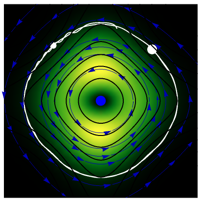
Here a very special transition is studied, which is a particle in a trigonometric two-dimensional Pöschl–Teller potential, where the transition goes from ground state (x,y) to a perturbed first excited superposition state (x,y)+a(x,y). Time-dependent transition effect in the Bohm approach was first described in[1]. This system is characterized by the fact that the trajectory varies between periodic and ergodic motion controlled by the factor . In phase space during the quantum flow, the velocity exhibits two nodal points (vortices) and two saddle points, due to the singularities of the wavefunction, which leads to a chaotic motion in the configuration space. Chaos or ergodic motion emerges from the scattering process of the trajectory with the nodal points[2].
Θ
0,1
Θ
1,0
Θ
0,0
a
Details
Details
Associated Legendre polynomials arise as the solution of the Schrödinger equation
-(+)ψ+-m(m+1)uy-n(n+1)uxψ=iℏψ
2
ℏ
2
m
p
∂
x,x
∂
y,y
2
sech
2
sech
∂
t
n=m=4
m
p
1
2
ℏ=1
∂
x
∂
∂x
Θ
0
Θ
1
it
E
0,1
e
(x)(y)+a(x)(y)
Θ
1
Θ
0
it
E
1,0
e
Θ
0
Θ
0
it
E
0,0
e
ψ=cos(Ωt)(x)(y)+isin(Ωt)(x)(y)+a(x)(y)
Θ
0
Θ
1
it
E
0,1
e
Θ
1
Θ
0
it
E
1,0
e
Θ
0
Θ
0
it
E
0,0
e
where (x), (y) are eigenfunctions, and are permuted eigenenergies of the corresponding stationary one-dimensional Schrödinger equation, with =+ and . In the wavefunction , the perturbation term is given by , where the parameter is an arbitrary constant. The eigenfunctions (x), (y) are defined by
ϕ
k
ϕ
j
E
k,j
E
k,j
E
k
E
j
a,Ω∈
ψ
a(x)(y)
Θ
0
Θ
0
it
E
0,0
e
a
ϕ
k
ϕ
j
Θ
k,j
Θ
k
Θ
j
-
(k-4)k!
(8-k)!
-
(j-4)j!
(8-j)!
4-k
P
4
4-j
P
4
where (x), (y) are associated Legendre polynomials. are the quantum numbers =+ with and . The wavefunction is taken from[3].
4-k
P
4
4-j
P
4
E
k,j
E
k,j
2
(k-4)
2
(j-4)
k,j∈
k,j<4
For , the velocity field obeys the time-independent part of the continuity equation (ρ)=0 with , where is the complex conjugate. For this special case (), the trajectory becomes strongly periodic, because of the sign changing for with of the velocity term.
a=0
∇
v
ρ=ψ
*
ψ
*
ψ
a=0
Ωt>
mπ
2
m>∈
In the program, if PlotPoints, AccuracyGoal, PrecisionGoal, and MaxSteps are increased (if enabled), the results will be more accurate.
References
References
[1] C. Dewdney and M. M. Lam, "What Happens during a Quantum Transition?," Information Dynamics (H. Atmanspacher and H. Scheingraber, eds.), New York: Plenum Press, 1991.
[2] C. Efthymiopoulos, C. Kalapotharakos, and G. Contopoulos, "Origin of Chaos near Critical Points of the Quantum Flow," Physical Review E, 79, 2009 036203. doi:10.1103/PhysRevE.79.036203, arXiv:0903.2655 [quant-ph].
[3] M. Trott, The Mathematica GuideBook for Symbolics, New York: Springer, 2006.
[4] G. Pöschl and E. Teller, "Bemerkungen zur Quantenmechanik des anharmonischen Oszillators," Zeitschrift für Physik, 83 (3–4), 1933 pp. 143–151, doi:10.1007/BF01331132.
[6] S. Goldstein. "Bohmian Mechanics." The Stanford Encyclopedia of Philosophy. (Jul 30, 2015) plato.stanford.edu/entries/qm-bohm.
External Links
External Links
Permanent Citation
Permanent Citation