In Ref. 1, the influence of several parameters for comfort (temperature, humidity, light in a room) was investigated using Box-Behnken matrices. Here, we reproduces some of the main results for model determination using LinearModelFit. In addition, statistical and ANOVA analyses are provided as well as contour and 3D plots shown on the same Figure.
coded values of the three factors
In[]:=
M={{-1,1,-1,1,-1,1,-1,1,0,0,0,0,0,0,0},{-1,-1,1,1,0,0,0,0,-1,1,-1,1,0,0,0},{0,0,0,0,-1,-1,1,1,-1,-1,1,1,0,0,0}}
Out[]=
{{-1,1,-1,1,-1,1,-1,1,0,0,0,0,0,0,0},{-1,-1,1,1,0,0,0,0,-1,1,-1,1,0,0,0},{0,0,0,0,-1,-1,1,1,-1,-1,1,1,0,0,0}}
In[]:=
Transpose@M//TableForm
Out[]//TableForm=
-1 | -1 | 0 |
1 | -1 | 0 |
-1 | 1 | 0 |
1 | 1 | 0 |
-1 | 0 | -1 |
1 | 0 | -1 |
-1 | 0 | 1 |
1 | 0 | 1 |
0 | -1 | -1 |
0 | 1 | -1 |
0 | -1 | 1 |
0 | 1 | 1 |
0 | 0 | 0 |
0 | 0 | 0 |
0 | 0 | 0 |
In[]:=
Dimensions[M]
Out[]=
{3,15}
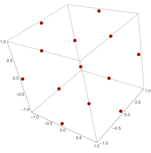
Visualize the design using Graphics3D
In[]:=
Show[Graphics3D[{Darker@Red,PointSize[0.025],Table[Point[Transpose[M][[i]]],{i,1,15}]}],Axes->True]
Out[]=
We assume the following comfort values (i.e., the responses)
In[]:=
yexp={3.0,3.4,3.4,3.0,5.0,4.0,4.4,4.4,8.2,8.3,8.2,8.1,9.4,9.2,9.3}
Out[]=
{3.,3.4,3.4,3.,5.,4.,4.4,4.4,8.2,8.3,8.2,8.1,9.4,9.2,9.3}
In[]:=
Dimensions[yexp]
Out[]=
{15}
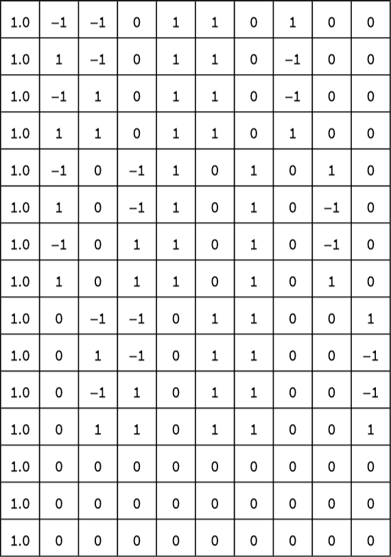
Forming MD (the Computation Matrix)
In[]:=
x1=M[[1]]
Out[]=
{-1,1,-1,1,-1,1,-1,1,0,0,0,0,0,0,0}
In[]:=
x2=M[[2]]
Out[]=
{-1,-1,1,1,0,0,0,0,-1,1,-1,1,0,0,0}
In[]:=
x3=M[[3]]
Out[]=
{0,0,0,0,-1,-1,1,1,-1,-1,1,1,0,0,0}
In[]:=
x1x1
Out[]=
{1,1,1,1,1,1,1,1,0,0,0,0,0,0,0}
In[]:=
x2x2
Out[]=
{1,1,1,1,0,0,0,0,1,1,1,1,0,0,0}
In[]:=
x3x3
Out[]=
{0,0,0,0,1,1,1,1,1,1,1,1,0,0,0}
In[]:=
x1x2
Out[]=
{1,-1,-1,1,0,0,0,0,0,0,0,0,0,0,0}
In[]:=
x1x3
Out[]=
{0,0,0,0,1,-1,-1,1,0,0,0,0,0,0,0}
In[]:=
x2x3
Out[]=
{0,0,0,0,0,0,0,0,1,-1,-1,1,0,0,0}
In[]:=
MD=Transpose[{{1.0,1.0,1.0,1.0,1.0,1.0,1.0,1.0,1.0,1.0,1.0,1.0,1.0,1.0,1.0},x1,x2,x3,x1x1,x2x2,x3x3,x1x2,x1x3,x2x3}];
In[]:=
Grid[Table[NumberForm[MD[[i,j]],{2,1}],{i,1,15},{j,1,10}],Frame->All,ItemSize->{2.7,2}]
Out[]=
Using LinearModelFit to get the model
In[]:=
Clear[x1,x2,x3]
In[]:=
data={MD,yexp}
Out[]=
{{{1.,-1,-1,0,1,1,0,1,0,0},{1.,1,-1,0,1,1,0,-1,0,0},{1.,-1,1,0,1,1,0,-1,0,0},{1.,1,1,0,1,1,0,1,0,0},{1.,-1,0,-1,1,0,1,0,1,0},{1.,1,0,-1,1,0,1,0,-1,0},{1.,-1,0,1,1,0,1,0,-1,0},{1.,1,0,1,1,0,1,0,1,0},{1.,0,-1,-1,0,1,1,0,0,1},{1.,0,1,-1,0,1,1,0,0,-1},{1.,0,-1,1,0,1,1,0,0,-1},{1.,0,1,1,0,1,1,0,0,1},{1.,0,0,0,0,0,0,0,0,0},{1.,0,0,0,0,0,0,0,0,0},{1.,0,0,0,0,0,0,0,0,0}},{3.,3.4,3.4,3.,5.,4.,4.4,4.4,8.2,8.3,8.2,8.1,9.4,9.2,9.3}}
In[]:=
lm=LinearModelFit[data,{1,x1,x2,x3,x1x1,x2x2,x3x3,x1x2,x1x3,x2x3}]
Out[]=
FittedModel
In[]:=
Normal[lm]
Out[]=
9.3-0.125x1-4.925x1x1-0.2x1x2+0.25x1x3+2.22045×x2-1.175x2x2-0.05x2x3-0.05x3+0.075x3x3
-16
10
statistical and ANOVA analyses.
A small p-value (typically < 0.05) means the variable significantly contributes to explaining the outcome.
A large p-value suggests the variable may not be important in the model and should be dropped from the model equation.
A small p-value (typically < 0.05) means the variable significantly contributes to explaining the outcome.
A large p-value suggests the variable may not be important in the model and should be dropped from the model equation.
In[]:=
lm[{"ParameterTable","RSquared"}]
Out[]=
,0.998451
Estimate | Standard Error | t-Statistic | P-Value | |
1 | 9.3 | 0.0983192 | 94.5899 | 2.50358× -9 10 |
x1 | -0.125 | 0.060208 | -2.07614 | 0.092515 |
x2 | 2.22045× -16 10 | 0.060208 | 3.68796× -15 10 | 1 |
x3 | -0.05 | 0.060208 | -0.830455 | 0.444113 |
x1x1 | -4.925 | 0.0886237 | -55.572 | 3.56876× -8 10 |
x2x2 | -1.175 | 0.0886237 | -13.2583 | 0.0000436266 |
x3x3 | 0.075 | 0.0886237 | 0.846274 | 0.436019 |
x1x2 | -0.2 | 0.0851469 | -2.34888 | 0.0656514 |
x1x3 | 0.25 | 0.0851469 | 2.9361 | 0.0324027 |
x2x3 | -0.05 | 0.0851469 | -0.58722 | 0.58257 |
In[]:=
lm[{"AdjustedRSquared","EstimatedVariance","ANOVATable"}]
Out[]=
0.995662,0.029,
DF | SS | MS | F-Statistic | P-Value | |
x1 | 1 | 0.125 | 0.125 | 4.31034 | 0.092515 |
x2 | 1 | 0. | 0. | 0. | 1. |
x3 | 1 | 0.02 | 0.02 | 0.689655 | 0.444113 |
x1x1 | 1 | 87.688 | 87.688 | 3023.73 | 3.76193× -8 10 |
x2x2 | 1 | 5.17852 | 5.17852 | 178.57 | 0.0000419831 |
x3x3 | 1 | 0.0207692 | 0.0207692 | 0.71618 | 0.436019 |
x1x2 | 1 | 0.16 | 0.16 | 5.51724 | 0.0656514 |
x1x3 | 1 | 0.25 | 0.25 | 8.62069 | 0.0324027 |
x2x3 | 1 | 0.01 | 0.01 | 0.344828 | 0.58257 |
Error | 5 | 0.145 | 0.029 | | |
Total | 14 | 93.5973 | | | |
3-D and contour plot for x3=0
In[]:=
Resp=9.3-0.125x1-4.925x1x1-0.2x1x2+0.25x1x3+2.22045*10^-16x2-1.175x2x2-0.05x2x3-0.05x3+0.075x3x3
Out[]=
9.3-0.125x1-4.925+2.22045×x2-0.2x1x2-1.175-0.05x3+0.25x1x3-0.05x2x3+0.075
2
x1
-16
10
2
x2
2
x3
In[]:=
x3=0;
In[]:=
p=ContourPlot[Resp,{x1,-1,1},{x2,-1,1},Contours->25,Axes->False,PlotPoints->30,PlotRangePadding->0,Frame->False,ColorFunction->"DarkRainbow"];
In[]:=
p3=Plot3D[Resp,{x1,-1,1},{x2,-1,1},ColorFunction->"DarkRainbow"];
In[]:=
level=0.0;gr=Graphics3D[{Texture[p],EdgeForm[],Polygon[{{-1,-1,level},{1,-1,level},{1,1,level},{-1,1,level}},VertexTextureCoordinates->{{0,0},{1,0},{1,1},{0,1}}]},Lighting->"Neutral"];Show[p3,gr,PlotRange->All,BoxRatios->{1,1,.9},FaceGrids->{Back,Left}]
CITE THIS NOTEBOOK
CITE THIS NOTEBOOK
Box-Behnken matrix for the optimization of comfort in a room
by Housam Binous and Ahmed Bellagi
Wolfram Community, STAFF PICKS, November 2, 2025
https://community.wolfram.com/groups/-/m/t/3569186
by Housam Binous and Ahmed Bellagi
Wolfram Community, STAFF PICKS, November 2, 2025
https://community.wolfram.com/groups/-/m/t/3569186