Wolfram Cloud Document

Meijer-G learning
by Sotirios Michos

This project explores the potential of the Meijer-G function to learn a black-box process and perform symbolic regression on a given set of data generated by such a process. The black-box process can be a system for which we have limited understanding, such as a neural network, or it can be any natural or artificial phenomenon that leads to the generation of data and for which we wish to increase our comprehension. The basis for this work is the referenced article where the authors propose a novel method for modeling data that comprises of the repetitive fitting of Meijer-G terms in order to capture the behaviour present in the data. The use of Meijer-G as a ridge function is motivated by its excellent analytic characteristics and its great expressibility that, especially for common functions, is usually achieved through only a small number of parameters. The same characteristics allow the Meijer-G based models to learn and reveal hidden information about the process that generated the data, ranging from an explanation of how the different factors contribute to the result to the actual law that generates the data. All these provide excellent interpolation and extrapolation capabilities that are highly sought after in modeling and regression analysis. In this project, we implemented the algorithm presented in the referenced article and utilizing the advanced optimization capabilities of Mathematica, we explore some key examples that illustrate both the power of this approach as well as recognize important issues and challenges that lay ahead and may lead to even greater future improvements.

Theory of the Meijer-G Function

The Meijer-G function is one of the most generic special functions that can express all the elementary functions as well as many advanced special functions like many kinds of Hypergeometric functions, Bessel functions etc. The main definition of the Meijer-G function employes a contour integration over the complex plane.

,...,

n+1

…,

,...,

m+1

,…,

2πi



Γ(1-

- s)…Γ(1-

- s)Γ(

+ s)…Γ(

+s)

Γ(

n+1

+s)…Γ(

+s)Γ(1-

m+1

-s)…Γ1-

-s

-s

where

0≤m≤q

and

0≤n≤p

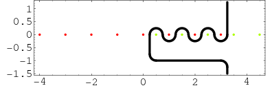
, for

and

are integer numbers, all the differences

for the various

i∈{1,...,n}

and

j∈{1,...,m}

and being non-integer and

z≠0

. There are many choices for the path of integration, one of which is shown in the following picture. The main idea in this choice if that the path comes from γ- ∞, for some real γ, and wiggle around the poles of the integrand in such a way that it leaves the (red) poles of the terms

Γ(

+ s)

for

i∈{1,...,m}

to the left and all (green) poles of the terms

Γ(1-

- s)

for

i∈{1,...,n}

to the right.

In order to see the scope of this function, we present some of the better known expressions that cover the usual elementary functions.



1,0

0,1

z



Sin(z)=

1,0

0,2

Sinh(z)=-



1,0

0,2

ArcTan(z)=

1,2

2,2

Log(1+z)=

1,2

2,2

z

1,1

1,0

.

Also, most of the advanced special functions are also supported like the lower and upper incomplete gamma functions

γ(a,z)

1,1

1,2

z

1,a



Γ(a,z)

2,0

1,2

z

a,0

,

the Bessel function of the first and second kind along with their modified variants

(z)=

1,0

0,2

(z)=

2,0

1,3

n+1

(z)=

-n



1,0

0,2

(z)=

2,0

0,2

as well as most hypergeometric functions like the Gauss’ hypergeometric function or even the generalized hypergeometric function

(a;b;z)

for

p>q+1

, of which it is a generalization.

(

;

;z)=

Γ(

)

Γ(

)Γ(

)

1,2

2,2

-z

,1-

0,1-

,...,

Γ(

)...Γ



Γ(

)...Γ(

)

1,p

p,q+1

-z

,...,1-

0,1-

,...,1-

In addition to this wide functional coverage, Meijer-G is characterized by excellent analytic properties like the h-th order derivative, being simply

,...,

n+1

…,

,...,

m+1

,…,

mn+1

p+1q+1

,...,

n+1

…,

,...,

m+1

,…,

as well as the celebrated convolution theorem

∞

∫

ηz

,…,

…,

μν

στ

ωz

,…,

z=

n+μ,m+ν

q+σ,p+τ

…,-

,…,

m+1

…,-

,…,

n+1

…,-

m+ν,n+μ

q+τ,q+σ

,…,

,…,-

n+1

…,

,…,-

m+1

…,

that allows for direct definite integration of a vast range of functions.

Meijer-G as a Symbolic Model

The properties presented in the previous section show that Meijer-G is an excellent function to be used for modeling, learning and symbolic regression purposes. In particular, when we are presented with a set of data, we are interested in finding a symbolic expression that fits the data as good as possible. Linear regression is the most prominent representative of this class of problems, where one tries to balance a line (or more generally a hyperplane) through the data in an optimal way to minimize the approximation error that is left out.

Symbolic regression is a more advanced kind of regression where, instead of trying to fit a simple line, one tries to discover the best symbolic expression among a particular class, that best approximates the data. If this class is large enough and contains the usual functions that commonly appear in practice, one can even hope to discover the actual law that generated the data. In this sense, Meijer-G has all the desirable characteristics in order to achieve this goal. It has a vast coverage of functions and can express all the common ones typically encountered in practical problems.

What is more, the Meijer-G is an analytic function over the whole complex domain, with the possible exception of the origin

z=0

and the unit circle

z=1

. That means that in the case of multidimensional data aggregated in its input, we can take its Taylor series and find out which factors contribute the most to each output. This is of fundamental importance in machine learning, as it may provide insights into how a black-box model (like a neural network) operates and which inputs affect a particular output. The authors of the referenced paper utilize this observation in order to propose an algorithm that attempts to build a superposition of Meijer-G functions that best fit the data generated by a neural network in order to explain its behavior. In the next section, we will present their algorithm with more details.

In this project, we implement the above algorithm in Wolfram Language and study it from the perspective of symbolic regression. In particular, we are interested in studying its behavior and assess its capability to model various kinds of data. Furthermore, we want to examine its capacity to discover the function that generated the data. For the purposes of this exposition within the time confines of the summer school, we limit ourselves to the study only some specific, simple examples that serve as a proof of concept for the suitability of Meijer-G in performing symbolic regression and also allow us to recognize some key issues, that need further investigation.

The Basic Theorem

The fundamental result showed in the referenced paper is that it takes only a small number of Meijer-G families in order to cover all the important functions. In particular, the theorem states that:

Consider the set of Meijer-G functions of the form



(z)=

,...,

n+1

…,

,...,

m+1

,…,

where

,...,

∈

;

r,s∈

and the hyperparameters belonging to the configuration set

(m,n,p,q)∈={(1,0,0,2),(0,1,3,1),(2,1,2,3),(2,2,3,3),(2,0,1,3)}

. This set of functions includes al the functions with the form

f(z)=Φ(w

)

with

w,l,t∈

;

Φ∈id,sin,cos,sinh,cosh,exp,log(1+.),arcsin,arctan,

1+.

,Γ

where

are the Bessel functions and

is Euler’s Gamma function.

In particular, the first family covers the functions

sin,cos,sinh

, and

cosh

, the second the

as well as the various monomials, the third the

exp

, and the gamma functions such as

, the fourth the

log(1+.),arcsin

and

arctan

, and the fifth the various Bessel function such as

and

The Fitting Algorithm: Symbolic Pursuit

The fitting algorithm is called symbolic pursuit and conceptually, it is very close to the well-known projection pursuit. The main idea is that we have an error or more properly a residual function whose norm expresses how far we are from actually capturing the data. What we to do then is an attempt to fit a model function to the residual, in order to “explain” a part of it, and make the residual as small as possible. The model function in our case is the Meijer-G function. Since our model function will typically be unable to fully explain the whole residual function, we repeatedly add more terms trying to further reduce (or “hunt down”) the residual, one step at a time and hopefully in the most optimal way possible. The process stops when the improvement in the residual has become too small (here we select a relative improvement of less that 10%), effectively meaning than what is left is probably beyond the reach of even a linear combination of our model functions. The reason for saying “probably” is because the optimization problem in each step is non-convex and the search surface may contain regions that have not been explored which may lead to better approximations than what we discovered.The way the method supports multidimensional data is by utilizing each Meijer-G function as a ridge function, passing the data first through an affine transformation before handing the over to the Meijer-G. The general form of the affine transformation is

+...+

, where the

are the coefficients of the transformation and the

are the individual features or factors of the data. However, since the authors of the paper try to avoid encounter or surpassing the unit circle in the complex plane, instead of this term they use the normalized form

<v,x>

v

which for data generated within the n-dimensional hypercube is guaranteed to be between 0 and 1. The

sing indicates that if the quantity is below zero, is taken to be zero. Of course, as we will see, this creates a series of issues for symbolic regression, such as not being able to capture the functional behaviour outside the hypercube (which can be partially remedied with normalizing the data) as well as not allowing particular forms of functions to be expressed. However, we opt to keep these limitations for now, since we are interested in giving a proof of concept of the method’s capabilities for symbolic regression and leave the various enhancements for the future.The detailed algorithm in pseudocode is presented in the supplemental material for the referenced paper so we will not give a detailed presentation where. However, we will go over the actual code line by line, explaining the intermediate steps and clarifying the implementation details of the algorithm.

Implementing Symbolic Pursuit

Our code first starts with initializing some helper structures and functions that allow us to easily build up and access the different Meijer-G families symbolically. In particular, H is a list of four associations giving the hyperparameters

(m,n,q,p)

for each family.

H=Association@@MapThread[Rule,{{"m","n","p","q"},#}]&/@{{1,0,0,2},{0,1,3,1},{2,1,2,3},{2,2,3,3},{2,0,1,3}};

Then we construct the function meijerG that accepts a single argument from 1 to 5, returning the corresponding Meijer-G function, with hyperparameters set to their corresponding family values and containing the parameters in symbolic form. The function returned is a pure function.

meijerG[f_]:=(MeijerG[{Table[

,{i,H[[f,"n"]]}],Table[

,{i,H[[f,"n"]]+1,H[[f,"p"]]}]},{Table[

,{i,H[[f,"m"]]}],Table[

,{i,H[[f,"m"]]+1,H[[f,"q"]]}]}//N,#]&);

The parameters in symbolic form for each Meijer-G function (including the coefficients of the affine transformation) are generated using the parameters function which accepts as arguments the Meijer-G family as well as the dimensions of the data.

parameters[f_,dim_]:=Flatten@{w,Table[

,{i,dim}],Table[

,{i,H[[f,"n"]]}],Table[

,{i,H[[f,"n"]]+1,H[[f,"p"]]}],Table[

,{i,H[[f,"m"]]}],Table[

,{i,H[[f,"m"]]+1,H[[f,"q"]]}]}

The final helper function is lossF that returns the loss for a particular Meijer-G term in symbolic form. The symbolic quantities are the Meijer-G parameters, the affine transform coefficients and the weight of the Meijer-G. The lossF function takes as arguments the explanatory variables, the corresponding value of the response variables (which typically are the values of the residual function) and the family of the used Meijer-G. Note that the Max function in the affine transformation is used to keep the computation away from a potential singularity at zero. The loss function that is evaluated and returned is the mean squared difference between the response and the estimated Meijer-G model values.

lossF[xTrain_List,yTrain_List,f_Integer]:=Module{dim,n,vVec,zVec,affine},dim=Length[xTrain[[1]]];n=Length[xTrain];(*AffineTransformCoefficients*)vVec=Table[

,{i,dim}];(*ExplanatoryVariables*)zVec=Table[

,{i,dim}];(*AffineTransform.*)affine=Max0.01,

vVec.zVec

Norm[vVec]Sqrt[dim]

;(*Returnthesymbolicloss.Thesymbolicvariablesaretheparameterstooptimize*)Mean@Table[

(yTrain[[i]]-wmeijerG[f][affine]/.MapThread[Rule,{zVec,xTrain[[i]]}])

,{i,1,n}]

The first important function of our implementation has the task to fit a single Meijer-G function to a particular set of data. It is called FitMeijer and expects as arguments the values of the explanatory variables in xTrain, the response (or residual function) values in yTrain, the families the Meijer-G over which to search for an optimal fit in fCheck and whether the search method should be done "Locally", "Globally" or using "Both" approaches. If these two arguments are not provided, the method will search among all the five families using both local and global search and return the best result it finds. Local and Global search is performed using Wolfram Languages’ own FindMinimum and NMinimize functions respectively. The authors of the referenced paper opt to use Conjugate Gradient Descent, but we choose to let Mathematica’s methods to decide the best optimization algorithm for each case. The user has also the option to define the accuracy and precision goals for the optimization methods using AG and PG, in order to tweak them towards better and slower or quicker but less accurate results. The default value we have selected for these arguments is 3 digits, which usually give a pretty good tradeoff between accuracy/precision and time. We give some additional explanations as comments in the code that follows. The function returns the chosen fitted term as a list containing the family, the loss, and a list of rules connecting the symbolic parameters to their optimal values.

One final issue we would like to comment is the command:

As we state in the relevant comment, this has been included to avoid some arithmetic inconsistencies we observed when working with the MeijerG function. In particular, during our experiments, we encounter the following MeijerG function.

Plotting this function returned the following erratic results:

However, rationalizing the parameters with high accuracy and re-evaluating them, lead to the correct output.

Key Examples

In this section, we provide some simple but key examples that illustrate how the method behaves for single and multi-dimensional symbolic regression and serve as a proof of concept for its potential.

A Linear Function

Discussion

We observe here the method faithfully capturing the symbolic expression, besides the low accuracy and precision settings. What is surprising is that local optimization works better than global optimization, which many times fail to yield the correct result. Currently, the method is rather slow, but given the fact that local optimization works so well, we can expect that there is a huge potential for further optimizations (the authors of the referenced paper themselves use the Conjugate Gradient Descent method, to perform the optimization). An intriguing point is the use of Rationalize[] to perform de-noising (here the noise is due to the low arithmetic accuracy/precision we selected). It is based on the reasoning that most forms of Meijer-G that reduce to simpler forms, have parameters that are either integers, half integers, or generally fractions involving small numerators or denominators. Thus, we expect that trying to approximate these parameters with a simple fraction has a good chance of revealing the underlying function that produced the data.

Sinus of Sqrt

In this example, we generate data from the composition of a sinus and square root function. The reason we are doing this is twofold. First, we would like to test the method against a more complex function. Secondly, a limitation of the algorithm as implemented in the referenced paper is that it does not search for powers of the argument or coefficients with a non-unity norm. This was done to avoid encountering singularities of the Meijer-G function. The result is that functions like Sin or ArcTan are left outside of the search space. Although we deem that this is acceptable for this proof of concept presentation of the algorithm, it is one of the key issues that need to be addressed in order to have an acceptably working version of the method and given that it can be supplemented quite easily, is one of the first improvement we are planning to include in the implementation.

We start again by generating the data. Note that, in order for the method the be exposed to the whole behavior of the function, we generated data beyond the usual interval, extending it over to [0,10]. This as we said before, has the risk of encountering singularities, that have to be taken into account in a full implementation. However, for this example, we did not encounter such issues. Also, AccuracyGoal and PrecisionGoal were left to their default values.

We proceed with fitting the model, using again a subset of the whole family to see how the algorithm will fare with the correct one.

Derive Meijer-G from fitted coefficients

The raw Meijer-G that was returned by the algorithm is:

Substituting, yields the correct result.

It is worth noting that FindFormula[], which is the system’s native function for performing symbolic regression fails to recognize the correct form (due to the low number of available data). So this means that the particular method may have to offer improvements to the way this system function works internally.

Discussion

In this example, we see the great potential of the method to capture more complex functional forms, but we also encountered the first obstacles that need to be addressed. In order for the sinusoidal form to be expressed, he had to go to a larger interval [0,10] and increase the AccuracyGoal/PrecisionGoal to their default values. The method increases the FindFormula[] capabilities but it has to be extended in order to account for pure trigonometric functions and be able to capture the whole expressive range of the basic theorem.

Logarithmic Function

Now we examine an interesting case, that although symbolically will not be recognized with local optimization, shows the great possibilities of this method for extrapolation. Again, we create 30 random sample points from our test function that we will feed to the method.

Fitting a Meijer-G yields the following result

Derive Meijer-G from fitted coefficients

The Meijer-G returned by the fitting algorithm is:

Here we observe something strange. The actual function is covered by the forth family, and it has the following expression

In contrast, we can compare the above result with the fitted MacLaurin expansion given by the FindFormula[] method.

Discussion

What we see in this example is that the Meijer-G fitting method, not only interpolates almost perfectly the correct function in the range [0, 1] but also extrapolates it exceedingly well! Although the end result does not discover the actual form of a function, the algorithm manages to find a set of different parameters that give an excellent fit to the given data, as well as beyond, up to an extend. In other words, we observe the big plasticity that characterizes the Meijer-G function, providing multiple ways of approximating and producing insights for a given dataset.

Approximating a two-term, two-variable function

In this example, we examine how the full method of successively fitting a new Meijer-G function and backfitting the previous terms works.

Fitted Meijer - G Model

The algorithm returns a sum of two fitted functions, one hypergeometric and one Meijer-G.
First, we see that the expression indeed corresponds to two terms, as before, but it is rather hard to acquire the exact simpler closed form of the functions, due to the two arguments being entangled within both terms. However, checking the accuracy of the fitted model we take the following result.

Discussion

What about Sin[z]?

Regression in the interval [0, 1]

Fitted Meijer - G Model

The algorithm returns a fitted Meijer-G of the first family, staying in deed close to the family that the trigonometric functions do reside.

This form can be simplified to a hypergeometric function if we Rationalize[] the terms themselves. However, what is interesting is to see the interpolation and extrapolation capabilities of the returned model.

The picture on the left, illustrates an excellent interpolation capability of the method, while the picture to the right shows that the model stops tracking the original function as soon as we step outside if the initial support of the dataset as soon as the “trend” of the sinus function changes.

Regression in the interval [0, 10]

In order to give a chance to the Meijer-G fitting algorithm to be exposed to the whole periodic nature of the sinus, we repeat the process for data generated over a larger interval.

Fitted Meijer - G Model

Now the algorithm take us to the third family, which typically covers the exponential and the gamma function. The model itself comprises of a single Meijer-G function.

The coefficient themselves show that it took a lot “squeezing around” this function to make it come close to the sinus. Plotting the function as before, however, will illustrate the quality of the result.

What we see here is that within the support of the dataset, the model manages to follow somewhat the behavior of the sinus function. However, as soon as it leaves the support it diminishes and goes to zero. In other words, both the interpolation as well as the extrapolation that is performed by this model are rather poor. These results illustrate the importance of extending the implementation to account for the trigonometric and other related functions.

Concluding remarks

In this project, we studied the utilization of the Meijer-G function as a symbolic model and its capability to learn and perform symbolic regression on a given dataset. We implemented two main functions, along with three helper functions. The first function fits a single Meijer-G to the given data and the second one iterated the first in a controlled manner in order to build a symbolic model comprise of a linear combination of Meijer-Gs. The method shows great potential for further development both towards modeling and understanding the generating process behind the data as well as towards discovering simpler closed-form expressions that may guide this process.

The immediate future direction for this method is to extend the basic model in order to cover the whole functional range presented in the basic theorem. Wolfram Language provides the following generalized form for the Meijer-G function which can be readily applied to implement this extension:

Furthermore, a parallel step that can be taken is the discovery of various heuristics that could make the optimization process run faster. The fact that local optimization and gradient descent methods yield such good results holds the promise of great potential gains with respect to optimization speed. Studying and further understanding the search space is expected to give important insights towards this direction.

Extending this method so that it robustly works outside the [0, 1] interval and handling the potential singularities is also of great importance, as it will allow it to capture long-range behaviours that are not expressed within the small confines of this integral and without having to perform normalization on the original data.

We saw how Rationalize was able to remove noise and let a Meijer-G function fall to a simpler for, revealing, in essence, the function that created the data. Having the ability to discover the law behind the data is one of the most appealing characteristics of using the Meijer-G function and a further exploration on discovering simpler closed forms that are “close” to the fitted parameters beyond Rationalize is a key future target.

Another important issue, relevant to the previous one, is the robustness of the method and its ability to yield useful results in the presence of noise. How noise affects its performance, what levels of noise can the method handle and its potential to perform denoising in a symbolic manner are all imperative questions.

During our experiments, we have encountered numerous cases where different families yield comparable results. This shows that there is an important overlap in the expressibility of each family. Studying this overlap and deciding which family is the more appropriate to choose for each case, so that the method as a whole may yield better results is also an important research venue.

The authors of the referenced paper proposed this method as a way to provide explainability of a black-box process, such as a neural network. Although we have not studied this aspect here, it is one of the most powerful characteristics of this approach to modeling. Being able to capture a wide range of phenomena, in a continuous manner and by a model containing only a few parameters holds the promise of potentially very important insights. In the referenced paper, Taylor expansion is proposed as a means to understand the non-linear contributions of factors to the end result, generalizing methods such as LIME that are able to talk about only linear dependencies. However, the Meijer-G function accepts a wide range of transformations such as Laplace and Fourier. This fact, along with it great ability to extrapolate from the given data may lead to further methods and even more advanced ways to provide explanations about the behaviour of a black-box process.

Keywords

◼

Symbolic Regression

◼

Machine Learning

◼

Meijer-G

◼

Symbolic Pursuit

◼

XAI

Acknowledgment

The author would like to thank Stephen Wolfram, for his insightful input to this project and the illuminating discussions that the author had the joy of participating. Furthermore, the author would like to express his gratitude towards his mentor Tuseeta Banerjee that supported and encouraged him throughout the Summer School, always providing thoughtful guidance and making sure the project’s goals would be realistic and compatible with the given timeframe. Also, Tigran Ishkhanyan was instrumental in bringing this work to fruition, lending his experience and discussing various important aspects with the author, assisting him to further realize the potential of this work and helping him along with Stephen and Tuseeta in selecting and prioritizing the various tasks among a wide range of options.

Finally, the author would like to express his deep appreciation and respect towards all the people behind the organization of Wolfram Summer School 2021: Mads Bahrami, Erin Cherry, Danielle Roman Mayer, the TAs Jesse Friedman and Daniel Sanchez, the multiple contributors to the online discussions and his dear classmates. Your support, enthusiasm, and approachability created a warm and inviting atmosphere that lead to maximum engagement with the school and provided the additional support needed to timely finish this work.

References

◼

https://proceedings.neurips.cc//paper/2020/hash/ce758408f6ef98d7c7a7b786eca7b3a8-Abstract.html