Exploring the rulial space of Boolean Networks, graphs associated with states that evolve following boolean functions. Finding Wolfram Class 4 behaviors in non-trivial Boolean Networks, leveraging ruliological methods and the Wolfram Science approach.
The Wolfram community spent much time studying Cellular Automata, seeing how their simple grids can generate immense complexity. Today I want to explore a slightly different kind of system: Boolean Networks. Instead of a rigid grid, we have a web of nodes. Each node has a state, 0 or 1. And at each step, each node looks at its connections and updates its state based on a simple logic rule. It is a minimal model of a “thinking” web, or perhaps a genetic regulatory network. How does such a system behave? Does it freeze? Does it become chaotic? Or can we find the kind of complex structured behavior that we see in biology and physics?
In[]:=
Get[CloudObject["user:matheo/BooleanNetworks.wl"]];
First Look
First Look
Let's start by observing a single, randomly generated Boolean Network. We pick a small number of nodes, say N=10. We decide that each node receives inputs from K=2 other nodes chosen at random. And for the logic, we just assign random truth tables to each node. It is not obvious that anything interesting should happen: one might expect pure noise or instant freezing. Here we visualize the network topology.
In[]:=
net=RandomBooleanNetwork[10,2];Topology[net]
Out[]=
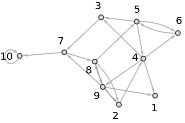
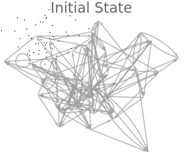
This shows the wiring, but the real story is in the dynamics. We will run the network for a given number of steps. It essentially means choosing an initial state and applying to it all the boolean functions to get the next state. Let's watch it evolve over time, and notice how quickly it settles into a pattern.
In[]:=
HistoryAnimation[net,RunBooleanNetwork[net,20]]
Out[]=
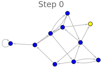
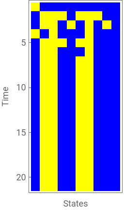
This evolving network visualization may feel convenient, but is actually highly inefficient to reveal any emergent structures or periodicity. Instead, I suggest using a state history matrix. It will serve as a visual reference to assess the richness of boolean networks. Columns of the matrix are nodes in the graph while rows are steps in time.
In[]:=
HistoryMatrix[net,RunBooleanNetwork[net,20]]
Out[]=
Varying Connectivity
Varying Connectivity
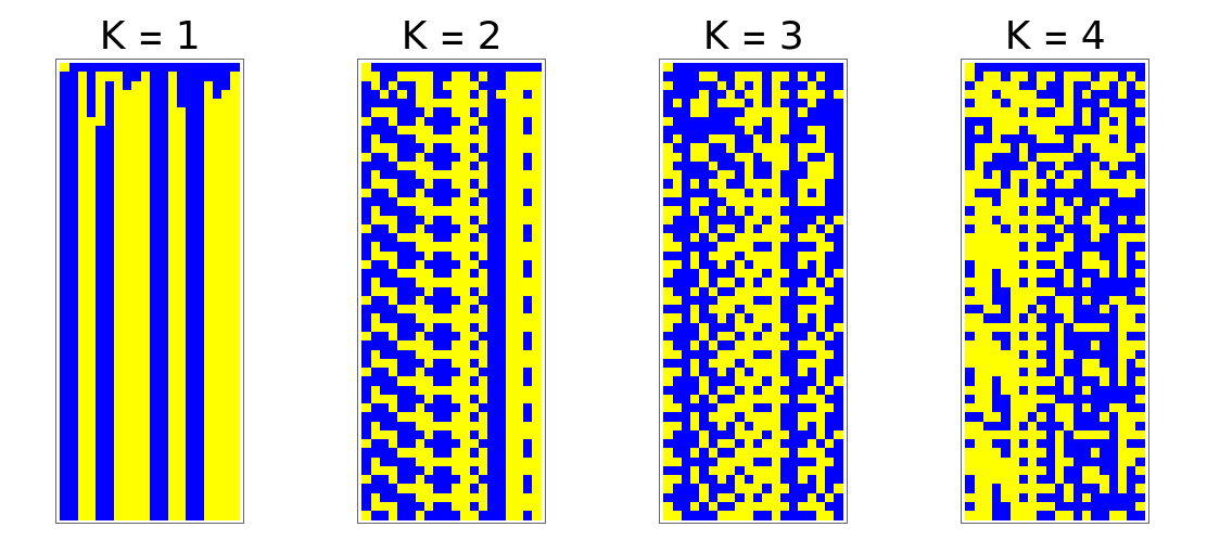
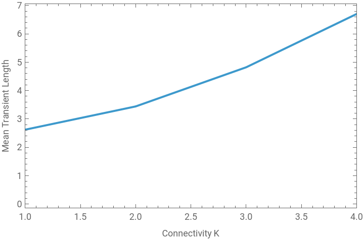
There is a parameter that seems to govern the 'temperature' of these systems: the connectivity K. In other words, it represents the number of inputs each node accepts. What happens as we turn this dial? If K=1, the network is sparse; information dies out, and the system freezes. If K=2, periodicity is quickly reached but a small amount of randomness emerges. If K>3, everything is chaotic, without any sense of compressibility.
In[]:=
KPlot[{1,2,3,4}]
Out[]=
This particular network (N=50, K=3) is illustrating the Frozen Core principle. Vertical lines are fixed points, preventing the entropy from corrupting the entire system. This equilibrium between chaos and order supposedly allows for computation, with enough stable nodes to act as a latent memory and enough active ones to adapt.
In[]:=
SeedRandom[55];Overview[RandomBooleanNetwork[50,3],100]
Out[]=

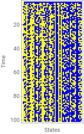
Notice that our networks evolve trough different states before reaching a fixed point. These are called the transient. Having a long transient essentially means not being trivial; however, every Boolean Network will eventually reach a state that has already been visited, which means periodicity is bounded by the amount of possible different states, 2^N.
In[]:=
TransientPlot[200,10,4,50]
Out[]=
About Universality
About Universality
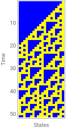
The Cellular Automata class is a strict subset of boolean automata. The only limit is that the latter are usually finite, but one can use a boolean network to compute any ECA up to an arbitrary number of steps, requiring N=steps. However, as demonstrated by Stephen Wolfram and Matthew Cook, some Cellular Automaton rules are universal. It proves that boolean networks can exhibit complex Wolfram Class 4 behavior, at least with K=3.
In[]:=
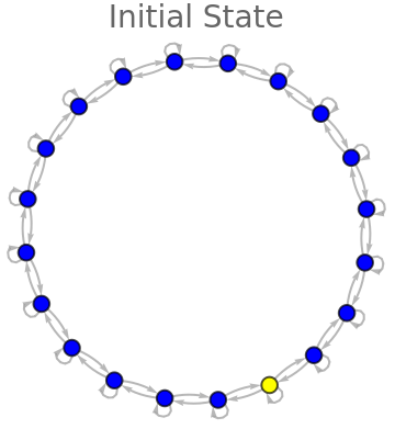
n=20;circularK3=Table[{Mod[i-2,n]+1,i,Mod[i,n]+1},{i,n}];Topology[r110]
Out[]=
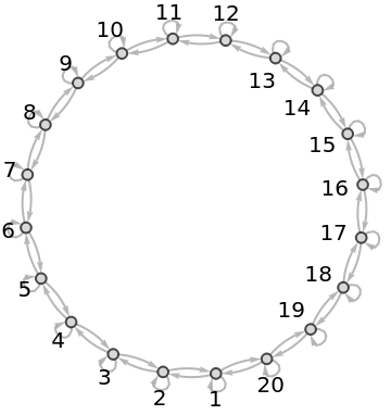
Here is the topology. We use a circular graph, with every node being influenced by its two 1D neighbors and itself. Its evolution over time is:
In[]:=
r110={circularK3,ConstantArray[110,n]};Overview[r110,50,2^(n-1)]
Out[]=
Informally speaking, computers are essentially fancy boolean automaton, with transistors and low-level code implementing K=2 rules. This is another evidence for the universality of these systems, but one could argue it might take huge values of N to see this property emerge. I’m skeptical about that.
Exhaustive Exploration
Exhaustive Exploration
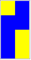
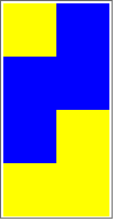
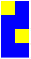
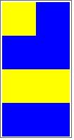
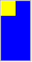
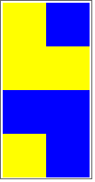
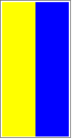
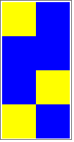
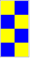
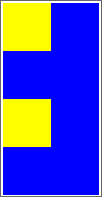
When I first introduced this essay to Stephen Wolfram, he emphasized the value of exhaustive search. Instead of guessing a clever design or attempting to sample a (very) large Rulial space, we will simply look at all possibilities for very small networks. By generating every possible network for 2, 3 or 4 nodes and finding their attractors (the loops the system eventually falls into), we are effectively cataloging the 'elementary particles' of this specific computational domain. Each attractor represents a distinct behavior available to the system.
In[]:=
ExhaustiveAttractors[2,1]
Out[]=
| | | | | | | |
In[]:=
ExhaustiveAttractors[2,2]
Out[]=
| | |
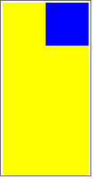
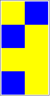
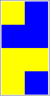
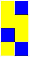
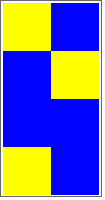
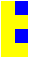
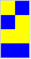
Let’s explore N=3 networks as far as we can. N=3, K=2 is already way too computationally expensive.
In[]:=
ExhaustiveAttractors[3,1]
Out[]=
| | | | | | | |
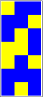
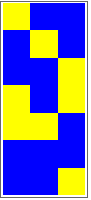
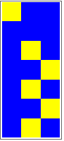
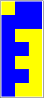
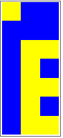
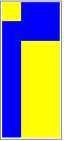
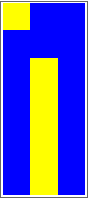
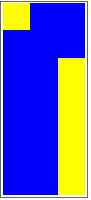
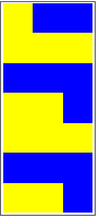
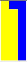
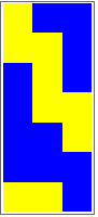
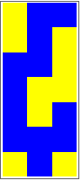
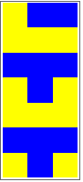
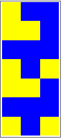
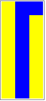
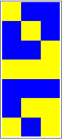
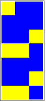
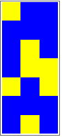
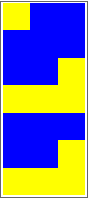
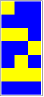
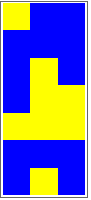
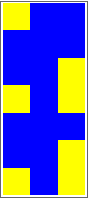
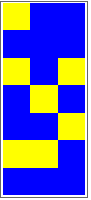
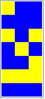
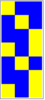
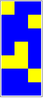
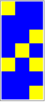
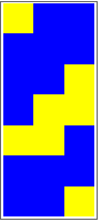
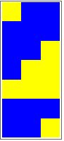
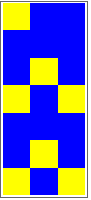
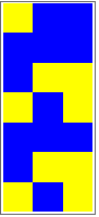
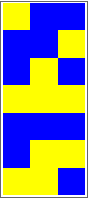
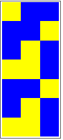
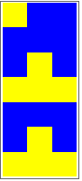
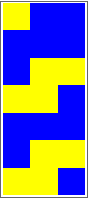
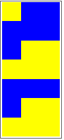
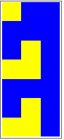
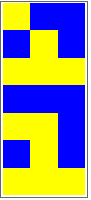
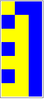
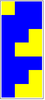
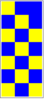
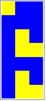
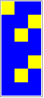
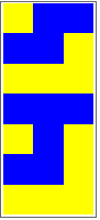
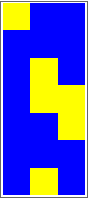
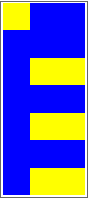
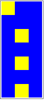
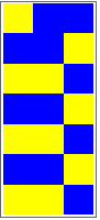
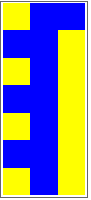
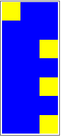
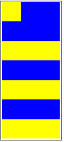
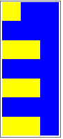
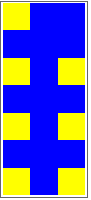
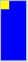
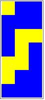
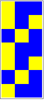
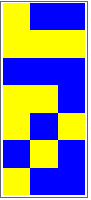
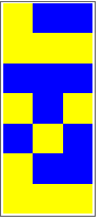
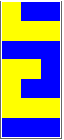
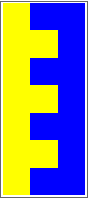
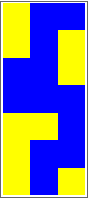
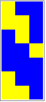
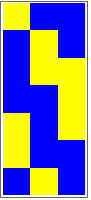
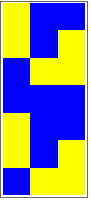
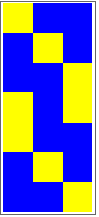
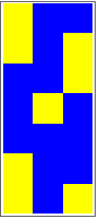
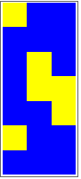
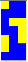
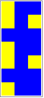
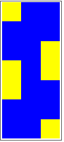
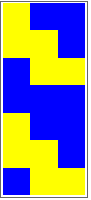
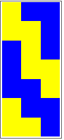
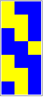
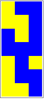
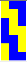
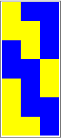
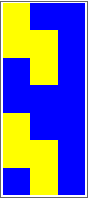
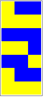
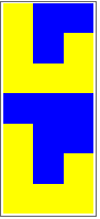
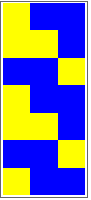
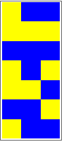
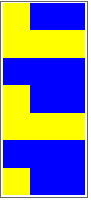
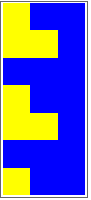
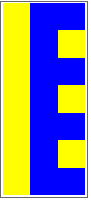
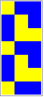
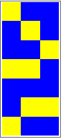
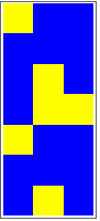
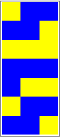
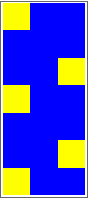
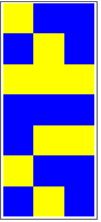
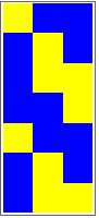
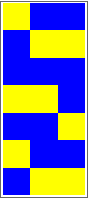
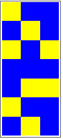
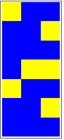
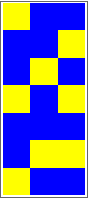
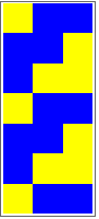
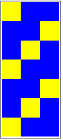
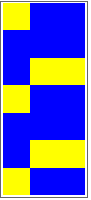
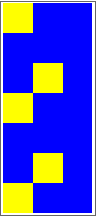
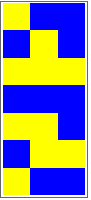
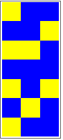
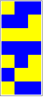
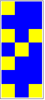
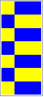
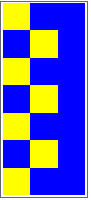
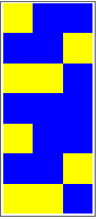
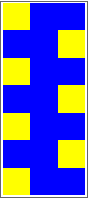
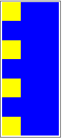
These are, in a sense, already extremely complex behavior showing a form of chaoticity, the best networks having a transient length of 7, which is near to the maximum periodicity. However, it feels a bit like cheating, because the space of possibilities is immense as we let K=2 and because K=1 is not nearly as intellectually satisfying. Let us focus on a specific slice of this space: networks where every gate is a NAND (the universal logic gate). It constrains the Rulial space, so that we can perform an exhaustive search on higher-K networks.
The same interesting patterns could emerge using XOR, known for its high chaoticity.
We can expand this search to include other gates. For instance, what is the interplay between AND and OR? These gates are monotonic, they don't 'flip' bits like NOT or XOR.
Notice that these gates are way less expressive than the previous ones. Here is the same exploration on N=4 networks:
Indeed, the XOR gates seems to generate the more various chaotic behavior. It resembles the rule 90 or 150 of Wolfram Elementary Cellular Automata, also based on the XOR gate. The diagonals we see on most of these indicate the network behaves like a counter (using the Linear Feedback Shift Register approach) and thus could be used to generate pseudo-random numbers. Now visualizing the attractors for N=4, NAND networks.
This is an interesting result. We see more organic patterns, with triangle-like structures and domain walls (cf. Frozen Core). Besides, the maximum transient length (8) we found is still not even close the 2^N=16, and the results are not providing enough evidence for universality, or, more generally speaking, class 4 behavior. What happens if we mix these two gates?
Notice this starts to resemble what we are looking for. What happens if we also constrain the topology space to a single dimension? It allows us to compute networks having way more nodes.
Using one-dimensional automatons, again, feels like cheating. These are effectively non-homogeneous cellular automata, having a “right-left” neighborhood with K=2. But, how about tweaking a little bit this circular wiring? For example, what would be the attractors of a butterfly-like network?
This is a huge evidence for Class 4 behaviour in general, random boolean networks. The minimal condition for it to appear clearly seems to be less related to K than to the number of nodes, because of the periodicity being bounded by 2^N. To make the demonstration even more convincing, let’s try to make the wiring non-planar so the boolean network if completely different from classical cellular automata.
The notion of information particles stays, and the same patterns are able to emerge. This is class 4 behavior, allowing for complex computation.
Biological Interpretation
Biological Interpretation
Why should we care about these abstract logical webs? It turns out nature has been building them for billions of years. The genes in a biological cell switch each other on and off with logic that looks remarkably like the networks we are studying. Real biological networks, however, are not chosen at random. They have been tuned by evolution. They often exhibit high 'Canalizing' properties (robustness), meaning that often the state of just one input is enough to determine the output, providing stability against noise. Let’s look at a real example (the control system for the Cell Cycle of Yeast) and see how it compares to our random samples. We can even calculate a 'BioScore' to measure how 'biological' its rules appear.
It turns out that this abstract mathematical behavior offers a profound model for biological differentiation. If we view the genome as a dynamic computational system, then the distinct cell types we observe in an organism (neuron, hepatocyte, skin cell) correspond precisely to these attractors. The cell effectively ‘computes’ its identity by traveling its state space until it falls into a stable cycle, locking it into a phenotype.
Acknowledgments
Acknowledgments
I want to address a huge thanks to my primary mentor Willem Nielsen for the enthusiasm and the various suggestions, to Eric Parfitt for the review and to Stephen Wolfram for the precious advices and support. Thanks to all the staff of the Wolfram Winter School for these two amazing weeks. I appreciated each lecture and each conversation, and it has been a pleasure participating in this event.
Further Directions
Further Directions
If I had some more time, I would have explored further the multiway causal graph visualisations. I would have tried more variations on the one-dimensional network showing interesting properties. One thing I didn’t manage to finish is the Adaptive Evolution part of this essay. I actually implemented it, but eventually chose to let it as future work.
References
References
1
.S. A. Kauffman (1969), “Metabolic stability and epigenesis in randomly constructed genetic nets,” Journal of Theoretical Biology.
2
.F. Li, T. Long, Y. Lu, Q. Ouyang, and C. Tang (2004), “The yeast cell-cycle network is robustly designed,” Proceedings of the National Academy of Sciences (PNAS).
3
.B. Derrida and Y. Pomeau (1986), “Random networks of automata: a simple annealed approximation,” Europhysics Letters.
4
.S. Wolfram (2002), A New Kind of Science. Wolfram Media.
CITE THIS NOTEBOOK
CITE THIS NOTEBOOK
Ruliology of Boolean networks
by Matheo Tripnaux
Wolfram Community, STAFF PICKS, January 15, 2026
https://community.wolfram.com/groups/-/m/t/3607574
by Matheo Tripnaux
Wolfram Community, STAFF PICKS, January 15, 2026
https://community.wolfram.com/groups/-/m/t/3607574