Intro
Intro
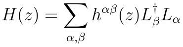
Following the work of “Objective Trajectories in Hybrid Classical-Quantum Dynamics.” (Oppenheim, Jonathan, Carlo Sparaciari, Barbara Šoda, and Zachary Weller-Davies. 2020. arXiv [Quant-Ph]. arXiv. http://arxiv.org/abs/2011.06009.), the master equation for Hybrid Classical-Quantum dynamics can be written using the positive rate matrix as follows:
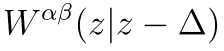

where is the classical phase-space point and are Lindblad operators encoding quantum jumps.




Unravelling the equation into trajectories at discrete steps of classical evolution with quantum jumps:

where probability to perform a quantum jump corresponding to a Lindblad term is proportional to :
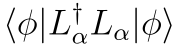
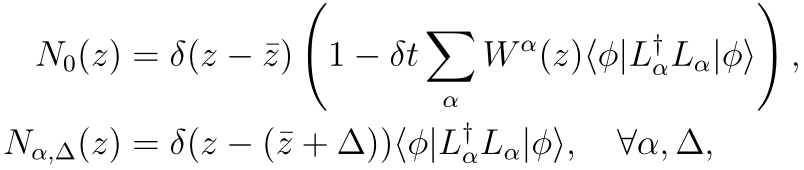

The mathematical equations do not matter much, the important point of the unravelling algorithm is that it can be turned into a simulation, at least in principle.
Bellow we define the SimulateCQTrajectories function to simulate two classic Stern-Gerlach and CHSH experiments using this hybrid approach.
Code
Code
Stern-Gerlach
Stern-Gerlach
For the Stern-Gerlach experiment we initialize CQ state with classical state for initial position and velocity of an electron and quantum superposition state :
z={q,p}={0,0}
|ψ〉=(|〉+|〉)
1
2
In[]:=
initState=<|"ClassicalState"->{0,0},"State"->{1,1}|>;
1
2
We assume that two possible quantum jumps corresponding to Lindblad operators =|0〉〈0| and =|1〉〈1|:
L
1
L
2
In[]:=
LindbladJumps=z|->
,
;
1 | 0 |
0 | 0 |
0 | 0 |
0 | 1 |
The classical coupling is assumed to be governed by linear Hamiltonian =∓z, and there the following gradients:
H
1,2
In[]:=
∇H=z|->{{-1,0},{1,0}};
With that we can simulate a number trajectories with some additional self-explanatory parameters:
In[]:=
SternGerlachResults=SimulateCQTrajectories[initState,"LindbladOperators"->LindbladJumps,"QuantumCouplingGradients"->∇H,"Iterations"->1000,"FinalTime"->1,"TimeStep"->.01,"JumpRate"->30.,RandomSeeding->123];
Plotting a small sample of trajectories shows that the quantum state quickly collapses at some random time step while kicking the particle in the corresponding direction and then continues kicking it in the same direction, therefor accelerating it:
In[]:=
positions=Normal@SternGerlachResults[;;5,All,{#"Time",#"ClassicalState"[[1]]}&];velocities=Normal@SternGerlachResults[;;5,All,{#"Time",#"ClassicalState"[[2]]}&];spins=Normal@SternGerlachResults[;;5,All,ExpectationValue[PauliMatrix[3]][#State]&];
In[]:=
GraphicsRow@ ListStepPlot[positions,AxesLabel->{"Step","z"}], ListStepPlot[velocities,AxesLabel->{"Step","v"}], ListStepPlot[spins,AxesLabel->{"Step","<>"}]
σ
z
Out[]=

As a result we detect an electron either going upward or downward:
In[]:=
ListPlot@Normal@SternGerlachResults[All,-1,#"ClassicalState"[[1]]&]
Out[]=
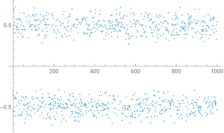
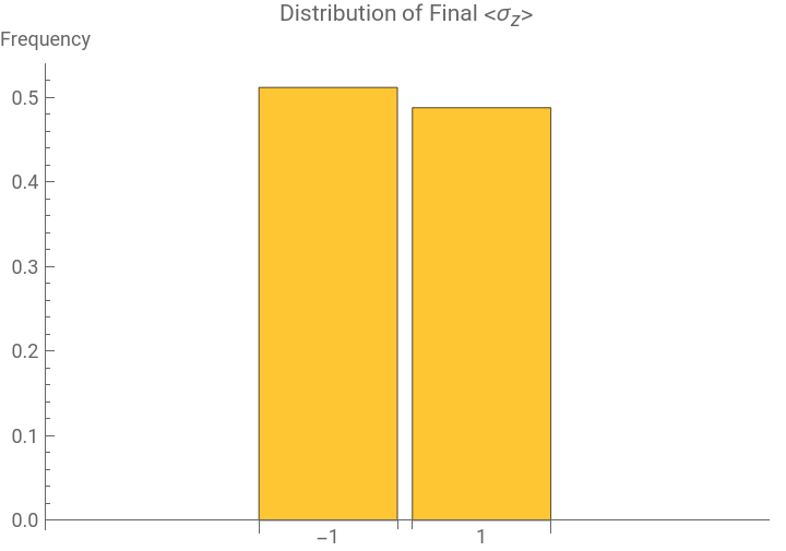
Showing roughly 50-50 split between the two:
Out[]=
Bell/CHSH
Bell/CHSH
Code
Code
Preparation
Preparation
There is a built-in maximally non-classical CHSH circuit:
In[]:=
<<Wolfram`QuantumFramework`
In[]:=
QuantumCircuitOperator["CHSH"][[;;-5]]
Out[]=
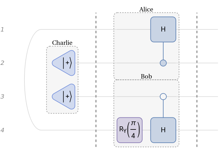
For simplicity we merge the rotation into the preparation state making it more spread out, but Alice’ and Bob’s operations become identical CH gates:
In[]:=
initState=QuantumOperator["RY"[-3Pi/4],{2}][QuantumState["PsiPlus"]]
Out[]=
1
2
1
2
2
)1
2
1
2
2
)1
2
1
2
2
)1
2
1
2
2
)In[]:=
initState["AmplitudePlot"]
Out[]=
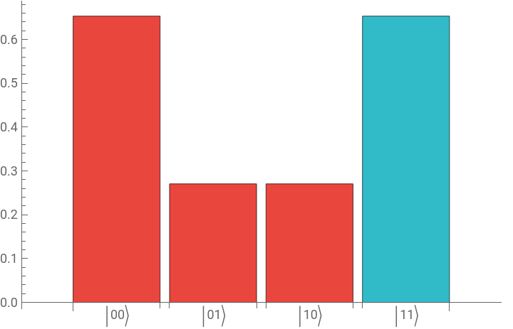
The resulting state and observables are the same:
We also split classical random choice, controlled by Charlie, into four different separately modeled scenarios corresponding to four combinations of measurement bases picked by Alice and Bob:
The overall set of parameters for simulating Hybrid Classical-Quantum system together with Lindblad and Coupling Gradients are as follows:
Simulation
Simulation
We simulate 500 trajectories with the above parameters:
Analysis
Analysis
There are four different types of classical trajectories particles can undertake, deflecting either upward or downward independent of the measurement settings:
Looking from above particles move straight with constant velocity, only encountering their corresponding deflectors in a narrow stripe:
Focusing on the trajectory ending in 00 quantum state, we can see that after the first particle got measured and kicked upward, probability of 10 and 11 final states plummet and probability of ending up in 00 or 01 increases:
Or in other words, particle kick in one location of space have influenced potential outcome of another particle instantly. This is the infamous non-local feature of quantum mechanics in action. Also the quantum state remains pure at any moment, its collapse happens randomly while detector’s field is active, which results in slight local jump of the classical state, which manifests itself as a tiny acceleration. Therefore this hybrid approach helps to clearly separate non-locality into only quantum degrees of freedom.
Aggregating the trajectories for all possible measurement settings we confirm that probability distributions for all possible outcomes have the desired shape:
write the concluding remarks, mention the possibility of simulating other setups, like double-slit

CITE THIS NOTEBOOK
CITE THIS NOTEBOOK
Simulating hybrid classical-quantum trajectories
by Nikolay Murzin
Wolfram Community, STAFF PICKS, April 26, 2025
https://community.wolfram.com/groups/-/m/t/3451033
by Nikolay Murzin
Wolfram Community, STAFF PICKS, April 26, 2025
https://community.wolfram.com/groups/-/m/t/3451033