ORIGINAL ARTICLE: Paul Cousin, Triangular Automata: The 256 Elementary Cellular Automata of the 2D Plane, arXiv:2309.15795 (2023). DOI: https://doi.org/10.48550/arXiv.2309.15795
Article Abstract: Triangular Automata (TA) stands for cellular automata in the triangular grid. This work focuses on the simplest type of TA called Elementary Triangular Automata (ETA). They are argued to be the two-dimensional counterpart of Wolfram’s Elementary Cellular Automata. Conceptual and computational tools for their study are presented along with an initial analysis. The paper is accompanied by a website where the results can be explored interactively. The source code is available in the form of a Mathematica package.
This Mathematica notebook introduces the topic of TA while demonstrating the functionalities of the Triangular Automata package.
Download this notebook: https://github.com/paulcousin/triangular-automata-mathematica
More information: https://paulcousin.github.io/triangular-automata
Download this notebook: https://github.com/paulcousin/triangular-automata-mathematica
More information: https://paulcousin.github.io/triangular-automata
Setup
Setup
Run the following command to import the package.
In[]:=
<<"https://paulcousin.github.io/triangular-automata-mathematica/TriangularAutomata.wl";
Introduction
Introduction
Cellular automata in the triangular grid, or Triangular Automata (TA) for short, have already been studied in a few papers [1-15]. This work will focus on a natural subset of TA called Elementary Triangular Automata (ETA).

ETA cells hold only binary states, each cell will thus either be:
◼
“alive” and colored purple , with a state

s=1
◼
“dead” and colored white , with a state

s=0
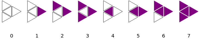
ETA rules determine the future state of a cell based on its current state and the states of its neighbors, regardless of their orientation. This results in only 8 possible local configurations. They can be plotted with TAConfigurationPlot.
In[]:=
GraphicsGrid@{TAConfigurationPlot/@Range[0,7],Range[0,7]}
Out[]=
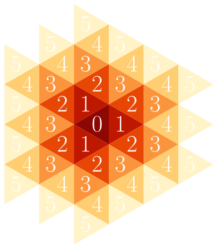
The package uses a graph-theoretical framework developed in a previous work on Graph-Rewriting Automata [18]. The triangular grid will here be considered as a graph. This graph must be expanded at each time step to simulate an infinite grid. The region of influence of a single cell grows in hexagonal layers. This is thus the most efficient way to expand the graph as well.
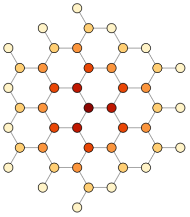
It is useful to see the triangular grid as a graph because computing the evolution of ETA is made quite easy by properties of its adjacency matrix and state vector . Every vertex v of this graph will hold a state s(v). The neighborhood N(v) of a vertex is defined as the set of its adjacent vertices.
ij
|
i
v
i
(
1
)The configuration of a vertex is a number which, when they are indexed as we previously did, can be expressed as follows:
c(v)
c(v)=4×s(v)+s(i)
∑
i∈N(v)
(
2
)The space of possible ETA rules is finite. For each one of the 8 configurations, a rule must specify whether the vertex will be dead or alive at . Consequently, there are only =256 possible rules. For this reason, ETA can be seen as the two-dimensional counterpart of Wolfram’s 256 Elementary Cellular Automata [16-17]. Furthermore, the triangle is the regular polygon tiling 2D space with the smallest number of neighbors per cell. ETA are thus the most basic 2D cellular automata and have a fundamental aspect in this regard.
Each rule R is a map from configuration space to state space.
t+1
8
2
Each rule R is a map from configuration space to state space.
R:{0,1,2,3,4,5,6,7}->{0,1}R((v))=(v)
c
t
s
t+1
(
3
)Each rule can be labeled by a unique rule number n. We will use the labeling system which was independently proposed in references [7] and [18], since it must be somewhat natural and because it has useful properties.
n=R(c)
7
∑
c=0
c
2
(
4
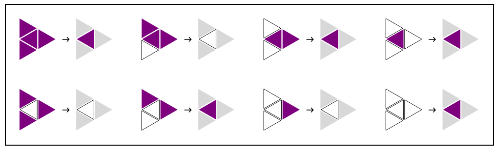
)This system, inspired by the Wolfram code [16], is such that a rule number in its binary form displays the behavior of the rule. Starting from the right, its digits indicate the future state for each configuration as they have been ordered previously. Rules can be plotted with the TARulePlot function.
In[]:=
TARulePlot[181,"Labeled"->True]
Out[]=
181 = 10110101 2 |
Basic functions
Basic functions
Starting Points
Starting Points
Grids have a special format. They are captured in a list with three elements: a precursor of the adjacency matrix, a state vector and a coordinates vector. The first two are in the SparseArray format.
To simplify things, this package provides few starting points ready to use:
To simplify things, this package provides few starting points ready to use:
1
.TAStartOneAlive: a grid with only one alive cell at the center
In[]:=
TAGridPlot@TAStartOneAlive
Out[]=

2
.TAStartLogo: a grid with a logo that contains all 8 local configurations.
In[]:=
TAGridPlot@TAStartLogo
Out[]=

3
.TAStartRandom[n]: a grid with cells that are randomly either alive or dead on n layers.
In[]:=
TAGridPlot@TAStartRandom[6]
Out[]=

Evolution
Evolution
We can evolve these grids with different rules using the function TAEvolve. Let’s try to evolve TAStartOneAlive with rule 181.
TAGridPlot@TAEvolve[TAStartOneAlive,181]
Out[]=

As expected from the earlier plot of rule 181, the environment has become alive and we have three dead cells surrounding a central alive cell. It would be nice to see what will happen after that. The function TANestEvolve can be used to jump ahead several time steps. Let’s look at what TAStartOneAlive will look like after 64 time steps of evolution with rule 181.
In[]:=
TAGridPlot@TANestEvolve[TAStartOneAlive,181,64]
Out[]=
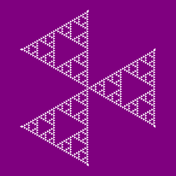
With this function, all the intermediate steps are lost and we only get the last grid. TANestListEvolve returns a list with all the intermediate steps.
In[]:=
GraphicsGrid@ArrayReshape[TAGridPlot/@TANestListEvolve[TAStartOneAlive,181,64],{8,8}]
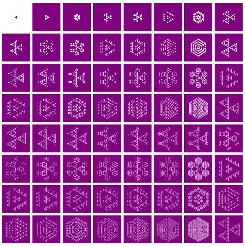
TAEvolutionPlot shows an animated version of what we have just computed.
Behavior
Behavior
In this section, a preliminary study of ETA is presented to motivate a future, more in-depth analysis. It is of particular interest to see what happens to a single living cell under different ETA rules so most of the following figures will come from this starting point.
Beauty
Beauty
One of the most striking aspects of these automata is their aesthetic quality, which cannot be better illustrated than by a few selected examples.
Chaos
Chaos
Given the existing literature on cellular automata, it is quite expected to see some of these rules behave chaotically. The example of rule 53 confirms it.
Starting from two randomly generated 64 layers wide grids that are completely similar except for the central cell, the trajectories strongly diverge.
Fractals
Fractals
Some ETA rules produce remarkable scale-free structures.
Space-Time
Space-Time
Similar to the way Elementary Cellular Automata [16-17] are most often represented, the evolution of an ETA can be displayed in one single plot. Here, an instant is two-dimensional, so adding the dimension of time creates a 3D structure. In these space-time plots, time flows downward. The successive grids are stacked beneath each other, starting from the initial conditions at the top. To avoid the infinite planes created by an alive environment, we can display only the cells that have the opposite state to it at each time step. A lot of information is therefore lost. We do not see most of the internal structure and we cannot know the state of the environment. Nevertheless, this representation helps visualize some properties of ETA that are difficult to notice otherwise. For instance, certain rules create 3D space-time fractals.
These plots can be exported to 3D software like Blender with the following code:
Self-Reproduction
Self-Reproduction
As mentioned in reference [15], one of the original motivations for the development of cellular automata was to create a mathematical model of self-reproduction. Interestingly, 4 of the 256 ETA rules naturally reproduce any finite pattern given as initial conditions: rules 85, 90, 165 and 170. A proof of self-reproduction based on path counting already exists for rule 170 [15]. Similarly spirited proofs could probably be proposed for the others.
Noise
Noise
Some rules seem to generate a pretty good noise. For example, if we pick a simple starting point without symmetries, rule 37 will usually turn it into an expanding disk with a random-looking interior.
Textures
Textures
Organic textures can be obtained by applying other rules to this pseudorandom grid.
Boring Rules
Boring Rules
There is an identity rule which leaves any grid unchanged: rule 240.
And a negative rule that swaps alive and dead states: rule 15.
Twins
Twins
A simple procedure can be followed to find the evil twin of a rule that has the same effect but in the negative world. To find it, take the number in its binary form (with the leading zeros needed for the number to be 8 digits long), swap ones and zeros and read it backwards. Let us take rule 214 as an example.
Two functions help work in the negative world: TANegativeGrid returns the negative of a grid and TANegativeRule returns the number of the twin rule.
Final Thoughts
Final Thoughts
If you want to delve deeper into the mathematics behind this work, you can read the related paper: https://arxiv.org/abs/2309.15795
I hope you will enjoy this package. Share what beautiful or interesting things you find with it!
References
References
◼
[1] C. Bays, “Cellular Automata in the Triangular Tessellation,” 1994.
◼
[2] L. Naumov, “Generalized coordinates for cellular automata grids,” in International Conference on Computational Science, Springer, 2003, pp. 869–878.
◼
[3] C. Bays, “Cellular Automata in Triangular, Pentagonal and Hexagonal Tessellations,” in Encyclopedia of Complexity and Systems Science, 2009, pp. 892–900.
◼
[4] Y. Lin, A. Mynett, and Q. Chen, “Application of Unstructured Cellular Automata on Ecological Modelling,” in Advances in Water Resources and Hydraulic Engineering, Berlin, Heidelberg: Springer Berlin Heidelberg, 2009, pp. 624–629. doi: 10.1007/978-3-540-89465-0_108.
◼
[5] C. Bays, “The game of life in non-square environments,” in Game of Life Cellular Automata, Springer, 2010, pp. 319–329.
◼
[6] B. Breckling, G. Pe’er, and Y. G. Matsinos, “Cellular automata in ecological modelling,” in Modelling Complex Ecological Dynamics: An Introduction into Ecological Modelling for Students, Teachers & Scientists, Springer, 2011, pp. 105–117.
◼
[7] M. Zawidzki, “Application of Semitotalistic 2D Cellular Automata on a Triangulated 3D Surface,” Int. J. DNE, vol. 6, no. 1, pp. 34–51, Jan. 2011, doi: 10.2495/DNE-V6-N1-34-51.
◼
[8] G. M. Ortigoza, A. Lorandi, and I. Neri, “ACFUEGOS: An Unstructured Triangular Cellular Automata for Modelling Forest Fire Propagation,” in High Performance Computer Applications, I. Gitler and J. Klapp, Eds., in Communications in Computer and Information Science, vol. 595. Cham: Springer International Publishing, 2016, pp. 132–143. doi: 10.1007/978-3-319-32243-8_9.
◼
[9] M. Saadat, “Cellular Automata in the Triangular Grid,” 2016.
◼
[10] S. Uguz, S. Redjepov, E. Acar, and H. Akin, “Structure and reversibility of 2D von Neumann cellular automata over triangular lattice,” International Journal of Bifurcation and Chaos, vol. 27, p. 1750083, 2017.
◼
[11] M. Saadat and B. Nagy, “Cellular Automata Approach to Mathematical Morphology in the Triangular Grid,” ACTA POLYTECH HUNG, vol. 15, no. 6, pp. 45–62, 2018, doi: 10.12700/APH.15.6.2018.6.3.
◼
[12] G. A. Wainer, “An introduction to cellular automata models with cell-DEVS,” in 2019 Winter Simulation Conference (WSC), IEEE, 2019, pp. 1534–1548.
◼
[13] A. V. Pavlova, S. E. Rubtsov, and I. S. Telyatnikov, “Using cellular automata in modelling of the fire front propagation through rough terrain,” IOP Conf. Ser.: Earth Environ. Sci., vol. 579, no. 1, p. 012104, Oct. 2020, doi: 10.1088/1755-1315/579/1/012104.
◼
[14] M. R. Saadat and B. Nagy, “Generating Patterns on the Triangular Grid by Cellular Automata including Alternating Use of Two Rules,” in 2021 12th International Symposium on Image and Signal Processing and Analysis (ISPA), Zagreb, Croatia: IEEE, Sep. 2021, pp. 253–258. doi: 10.1109/ISPA52656.2021.9552107.
◼
[15] M. R. Saadat and N. Benedek, “Copy Machines - Self-reproduction with 2 States on Archimedean Tilings,” 2023.
◼
[16] S. Wolfram and others, A New Kind Of Science, vol. 5. Wolfram media Champaign, IL, 2002.
◼
[17] E. W. Weisstein, “Elementary Cellular Automaton”, [Online]. Available: https://mathworld.wolfram.com/ElementaryCellularAutomaton.html
◼
[18] P. Cousin and A. Maignan, “Organic Structures Emerging From Bio-Inspired Graph-Rewriting Automata,” in 2022 24th International Symposium on Symbolic and Numeric Algorithms for Scientific Computing (SYNASC), Hagenberg / Linz, Austria: IEEE, Sep. 2022, pp. 293–296. doi: 10.1109/SYNASC57785.2022.00053.
CITE THIS NOTEBOOK
CITE THIS NOTEBOOK
Triangular Automata: The 256 Elementary Cellular Automata of the 2D Plane
by Paul Cousin
Wolfram Community, STAFF PICKS, October 17, 2023
https://community.wolfram.com/groups/-/m/t/3050730
by Paul Cousin
Wolfram Community, STAFF PICKS, October 17, 2023
https://community.wolfram.com/groups/-/m/t/3050730