This project utilized the Pixet particle detector to study various properties of cosmic rays. Several experiments were conducted investigating radiation shielding and the source of the incoming particles. The Poisson Distribution was explored to model the random independent cosmic rays. To find the main source of the incident particles, the frequency of particles was correlated to the solar irradiance to give firm basis to the assumption that most measured particles originated from the sun. Then to explain an anomaly in observations, the stopping power of the clouds for various particles was calculated.
Introduction
Introduction
Particle detectors play a central figure in the history of physics. In the early days of particle physics, detectors like cloud chambers and bubble chambers were used to detect particles and study their properties . These detectors relied on particles leaving visible trails in supersaturated vapor.
Later, as particle accelerators grew in size and power, massive detectors were built to study the new particles being created . The Large Hadron Collider at CERN contains massive detectors like the 7, 000 tonne ATLAS detector, collecting petabytes of collision data per second.
Through the pixel detector, fitting within the palm of my hands, I have attempted to perform experimental physics - collect data, form hypotheses and come to conclusions.
Semiconductor detectors incident particles by counting the charge carriers released between two electrodes in the detector material. When a charged particle passes across the semiconductor it will excite electrons - creating electron-hole pairs. As the amount of energy required to create an electron-hole pair is known, and is independent of the energy of the incident particle, measuring the number of electron-hole pairs allows the energy of the incident particle to be determined.
Pixel Detectors consists of individual units - silicon pads which allows us to know the position of the incident particles. Particles can either hit the surface of the detector perpendicularly, creating dots on the pixel detectors or come at an angle, leaving behind its path.
Pixel Detectors consists of individual units - silicon pads which allows us to know the position of the incident particles. Particles can either hit the surface of the detector perpendicularly, creating dots on the pixel detectors or come at an angle, leaving behind its path.
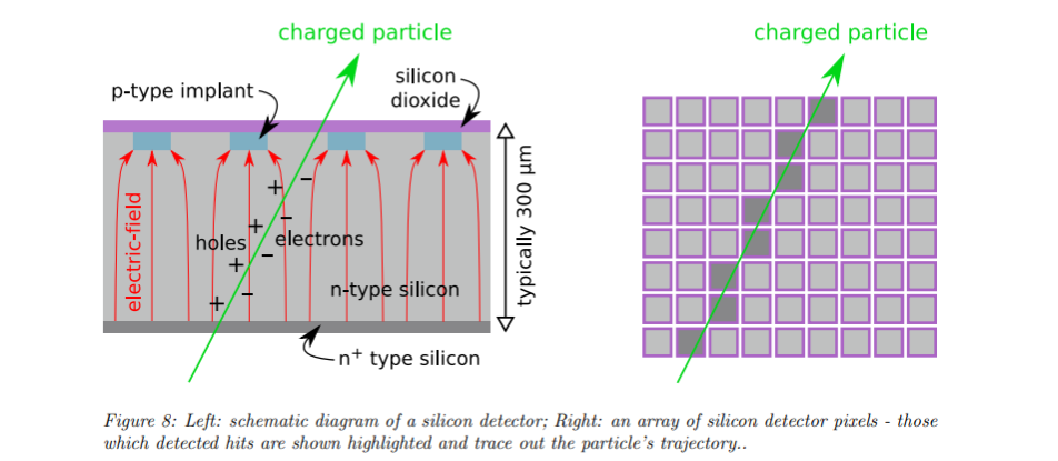
The detector I used was the MINIPIX EDU. The silicon detector consists of 256 x 256 pixels with pitch of 55 μm and 300 μm thick silicon.
Constraints
1. Lack of Calibration:
A calibrated detector would provide energy values that would correspond to units of physics. Without such calibration, only a statistical analysis can be performed.
2. 2-Dimensional Detector
Pixel detectors are often measured in several layers to gain 3-dimensional path of the incident particles. Having only a 2D detector does not provide the path of the particles.
3. Time to collect Data
Due to the limited time given for completing this project, taking quantitative measurements over a long period of time was not an option which would have decreased random variance due to external sources.
Data Preprocessing
Data Preprocessing
The Software for the MiniPIX detector exports two class of data -
◼
Spacial Data - Provides the position of the pixel pad which detected particles. This data is also temporal, providing each measurements taken after a set time interval(1 second).
◼
Spectra Data - Provides a histogram with - Energy, Time and Size on the x-axis with the number of particles on the y-axis .
Spatial Data
Spatial Data
The Pixet detector has a 256x256 individual silicon pads that measure incoming particles. I converted the raw data to a 256x256 Matrix and then to an image, where each pixel in the image corresponds to an individual silicon pad of the detector.
Function to turn the .txt file to a 256x256 Matrix.
In[]:=
toMatrix[file_] := Partition[Flatten [ToExpression/@StringSplit[#] &/@{file}], 256]
Extracting Data from raw data files.
SumImage = CloudGet["https://www.wolframcloud.com/obj/c96adb21-c6f8-417b-a7de-6e2119903024"];
Plot the Matrix of the Incident Particles
In[]:=
Image[MatrixPlot[SumImage]]
Out[]=
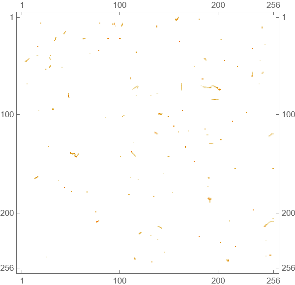
These tracks and dots represent the particles incident on the particle detector, where each pixel corresponds to the the individual pads. When an incident particle comes at and angle, it excites several different pads which allows a track to be observed. The different colors represents the varying energy levels of the particles.
We can better observe the intensity of the incident particles by viewing a 3D model of the detector.
We can better observe the intensity of the incident particles by viewing a 3D model of the detector.
Plot the 3D Graph.
ListPlot3D[SumImage,ColorFunction->"DarkBands"]
Out[]=

Sum up all the frames
In[]:=
listOfMatrices=toMatrix /@ texts;frames=Image[Table[Image[listOfMatrices[[n]]],{n,1,Length[listOfMatrices],1}]];
Plot a Video of the collected particle tracks
In[]:=
CloudGet["https://www.wolframcloud.com/obj/fe3025cc-d15d-481e-b394-90004cddaea1"]
Out[]=
Spectra Data
Spectra Data
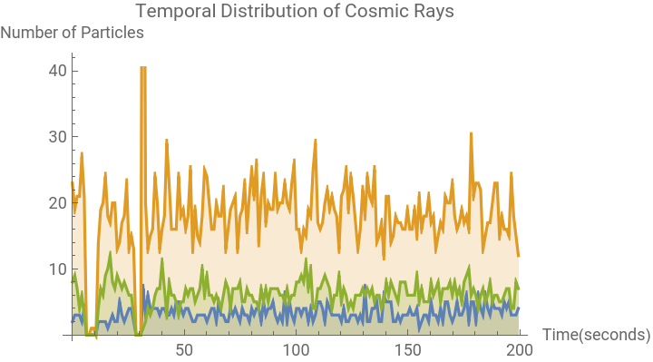
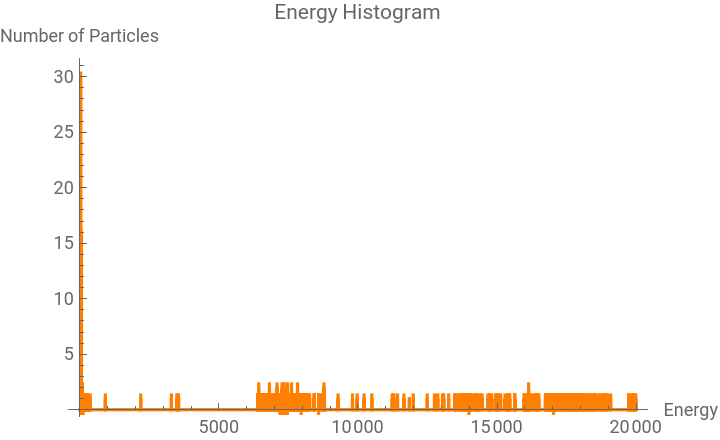
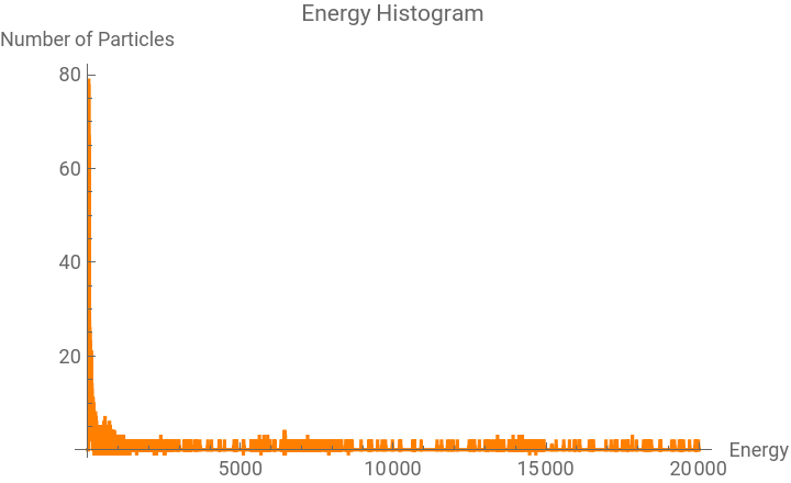
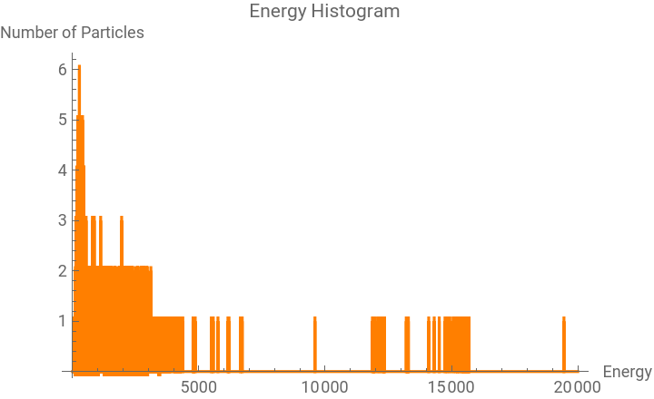
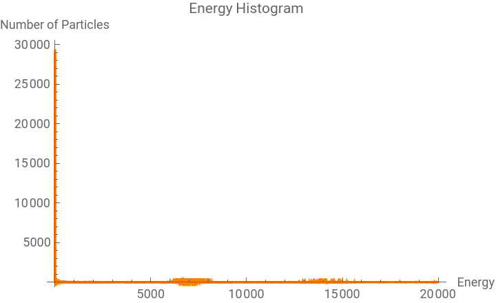
The Pixet software also exports “Spectra” data. It provides a histogram with - Energy, Time and Size on the x-axis with the number of particles on the y-axis . It does this for every particle type that it detects - Alpha Particle, Electron, Muon, Photon.
The Timeline histogram provides the number of particles at a time t. The Energy histogram provides the number of particles with a certain energy level, but the unit of the energy is not specified, and requires calibration with a constant known source. The Size histogram provides the number of particles with a certain size, without specifying the units or measurement magnitude.
The Timeline histogram provides the number of particles at a time t. The Energy histogram provides the number of particles with a certain energy level, but the unit of the energy is not specified, and requires calibration with a constant known source. The Size histogram provides the number of particles with a certain size, without specifying the units or measurement magnitude.
Get the Spectra Data from the raw data files
In[]:=
getSpectra[file_] := Module[{data=Flatten[CloudImport[file, "Table"]]},Return[Transpose/@Partition[Partition[data,(data//Length)/8],2]]];
dataPoints = getSpectra["https://www.wolframcloud.com/obj/ypragyan2021/11-1/T.txt"];ListLinePlot[Table[dataPoints[[i]], {i,{1,2,3}}], Filling->Axis, PlotLegends{"Alpha","Electron","Muon"}, PlotLabel -> "Temporal Distribution of Cosmic Rays", AxesLabel->{"Time(seconds)", "Number of Particles"}]
Out[]=


In[]:=
dataPoints = getSpectra["https://www.wolframcloud.com/obj/ypragyan2021/11-1/E.txt"];energyplots = {ListLinePlot[dataPoints[[#]], Filling->Axis, ImageSize-> "Medium", PlotStyle->Directive[Orange], PlotLabel->"Energy Histogram", AxesLabel->{"Energy", "Number of Particles"}] &/@{1,2,3,4}}
Out[]=
,
,
,
Morphological Analysis
Morphological Analysis
To further analyse the graphical data, I attempted to extract the morphologically similar structures and classify them based on their size. First I perform image preprocessing than find the morphological components, detect the components’s edges and then their areas.
Looking at the above graphs, infer the angular distribution of the incoming particles. There are many more particles being detected as dots than as large tracks(74 large tracks and 13 small tracks). This is due to the fact that very few particles hit the detector at an angle such that it is detected by multiple silicon pads and forms large tracks.
Poisson Distribution
Poisson Distribution
Statistics
Statistics
Discovering structure in randomness.
The Poisson distribution is a discrete probability distribution that expresses the probability of a given number of events occurring in a fixed interval of time or space if these events occur with a known constant mean rate and independently of the time since the last event.
The Poisson distribution is a discrete probability distribution that expresses the probability of a given number of events occurring in a fixed interval of time or space if these events occur with a known constant mean rate and independently of the time since the last event.
Lambda (λ) is the mean number of events within a given interval of time or space. For this application of the Poisson distribution the time interval is 1 second.
Poisson Distribution of Cosmic Rays
Poisson Distribution of Cosmic Rays
Here I plot the Poisson distribution based on the mean number of particles observed. Then I plot the Histogram of the observed values. The distribution should cosmic rays follow a Poisson distribution because the arrival of these particles is a random process and each arrival of each particle is independent of each other, but here it can be observed that the observed data does not fully follow the probability distribution.
Once possible reason, could be that each particle type follows its own Poisson Distribution.
Once possible reason, could be that each particle type follows its own Poisson Distribution.
Floor Shielding
Floor Shielding
The intention of this experiment was to find a correlation between the radiation shielding at different floors of a building. My hypothesis was that there would be a greater number of particles measured on the 4th floor than the 1st floor. I formed this hypothesis because I had assumed that the floors of the buildings would act as shielding for the cosmic rays as they are made from concrete(a good radiation shielding material) and the 1st floor would have a greater amount of shielding.
But there was no meaningful statistical difference between the number of observed particles at both the floors.
But there was no meaningful statistical difference between the number of observed particles at both the floors.
Solar Correlation
Solar Correlation
Theory
Theory
Temporal Correlation of Cosmic Ray Propagation
Temporal Correlation of Cosmic Ray Propagation
As is evident from the graph above, the number of particles peak at 1:00 (daylight saving), which gives firm basis for assuming that the sun is the main source of the particles detected.
We also observe that the alpha particles follow the solar irradiance,
Cloud Shielding Anomaly
Cloud Shielding Anomaly
Observation
Observation
These measurements were taken outside at 10:00 when a cloud passed over the detector, significantly reducing the amount of particles detected. But then an interesting anomaly was observed. The detection all 3 particles types - Electrons, Muons, Photons dropped, but the Alpha particles measurements did not show a significant dip.
Import the data and plot the temporal distributions of all the particles except photons(too many)
Plot the temporal distributions of individual particles.
Stopping Power
Stopping Power
Find the Power loss of an Alpha Particle in water
Find the Power loss of an Alpha Particle in Water
Bar Chart, showing the different in magnitudes of the loss of energy of alphas and electrons in a cloud.
As is evident from the graph, there is a difference in magnitudes between the stopping power of clouds for alpha particles and the electrons. This explains why the alpha particles did not show any dip in the measurements when the cloud passed over the detector as compared to other particles.
Future Work
Future Work
◼
Future work in this area could explore the radiation shielding of cosmic rays by clouds by adopting more complex simulations for the radiation shielding.
◼
Radiation Shielding by floors of a building could be further explored by collecting measurements taller buildings.
Acknowledgements
Acknowledgements
I would like to thank my mentor Daniele Ceravolo for his support to the development of this project.
CITE THIS NOTEBOOK
CITE THIS NOTEBOOK
Analyzing cosmic rays using the Pixet particle detector
by Pragyan Yadav
Wolfram Community, STAFF PICKS, July 13, 2023
https://community.wolfram.com/groups/-/m/t/2965243
by Pragyan Yadav
Wolfram Community, STAFF PICKS, July 13, 2023
https://community.wolfram.com/groups/-/m/t/2965243