In this short computational essay, I will explore the quantum adder circuits. I shall briefly implement classical half-adder, full-adder and Ripple-Carry adder in the conventional way (ie, classical). Then I will implement the quantum versions using the Wolfram Quantum Computation Framework.
Introduction
Introduction
For more details, I refer the reader to the Wikipedia entry on Adder, or this free textbook: Introduction to Classical and Quantum Computing. For the quantum circuit designs, I have used some circuits discussed in the section 4.5 “Quantum Adders” of the mentioned textbook. The notation that I am using here for the bitwise operations are different from the one in Wolfram. For example, for XOR, I will use A⊕B, instead of A⊻B.
Classical Half-Adder
Classical Half-Adder
The half-adder can be define as HalfAdder[A,B]={C,S} with S=A⊕B and C=AB
In[]:=
HalfAdder[A_,B_]:={BitAnd[A,B],BitXor[A,B]}
The truth table for the half adder:
In[]:=
<|{"A","B"}->{"C","S"},AssociationMap[Apply[HalfAdder],Tuples[{0,1},2]]|>//Dataset
Out[]=
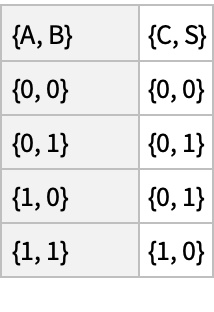
Quantum Half-Adder
Quantum Half-Adder
The quantum version of half-adder
In[]:=
qHalfAdder=QuantumCircuitOperator[{QuantumOperator["Toffoli"],QuantumOperator["CNOT",{1,4}],QuantumOperator["CNOT",{2,4}]}];qHalfAdder["Diagram"]
Out[]=
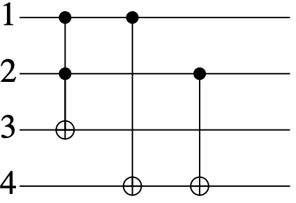
Note that the quantum circuit operator in our framework is defined completely independent from any given initial state. for pedagogical purposes, one can add the corresponding states (initial and even final) into the circuit diagram
In[]:=
qHalfAdder["Diagram","WireLabels"->{{Placed["A",Right],Placed["A",Left]},{Placed["B",Right],Placed["B",Left]},{Placed["C",Right],Placed["0",Left]},{Placed["S",Right],Placed["0",Left]}}]
Out[]=
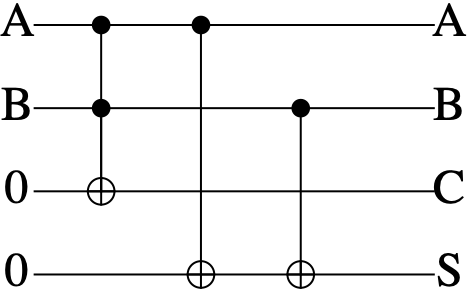
Setting ancillary qubits as zero, and consider all combinations for A and B:
In[]:=
states=QuantumState[StringJoin[#,"00"]]&/@Tuples[{"0","1"},2];
Applying the circuit, then measuring qubit 3 and 4 (note measurement step can be added into the circuit, too; only for simplicity, we did not do so):
In[]:=
final=QuantumMeasurementOperator[{3,4}][qHalfAdder]/@states;
Return corresponding measurement probabilities:
In[]:=
#["Probabilities"]&/@final
Out[]=
{|00〉1,|01〉0,|10〉0,|11〉0,|00〉0,|01〉1,|10〉0,|11〉0,|00〉0,|01〉1,|10〉0,|11〉0,|00〉0,|01〉0,|10〉1,|11〉0}
As one can see, for each case, one gets uniquely one outcome (one measurement result with nonzero probability).
In[]:=
Keys[DeleteCases[#["Probabilities"],0]]&/@final//Flatten
Out[]=
{|00〉,|01〉,|01〉,|10〉}
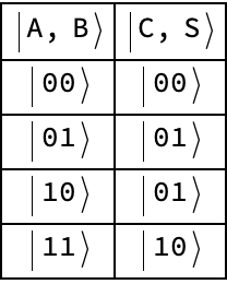
The truth table for the quantum half adder :
In[]:=
Grid[Prepend[Transpose[{QuantumState[#]["Formula"]&/@StringJoin@@@Tuples[{"0","1"},2],%}],{"|A,B〉","|C,S〉"}],FrameAll]
Out[]=
Classical Full-Adder
Classical Full-Adder
The full-adder can be implemented as follows where single-bit numbers A and B are added, the result is S, together with a carrier .
C
out
FullAdder[,A,B]={S,
C
in
C
out
S=A⊕B⊕C
C
out
C
in
In[]:=
FullAdder[Cin_,A_,B_]:={BitXor[A,B,Cin],BitOr[BitAnd[A,B],BitAnd[Cin,BitXor[A,B]]]}
Note that in order to build the full-adder, we have used 5 logic gates (i.e., 5 built-in WL functions). That is important for the circuit complexity.
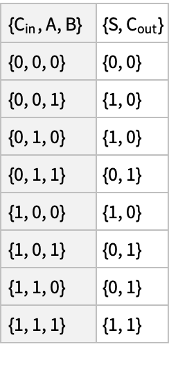
The truth table for the full adder:
In[]:=
<|{"","A","B"}->{"S",""},AssociationMap[Apply[FullAdder],Tuples[{0,1},3]]|>//Dataset
C
in
C
out
Out[]=
Quantum Full-Adder
Quantum Full-Adder
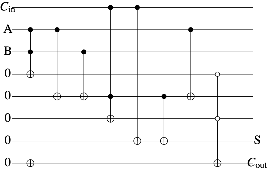
Here we discuss the quantum version of classical full-adder. Note we are dealing with only single bit numbers, for now.
In[]:=
qFullAdder=QuantumCircuitOperator[{QuantumOperator["Toffoli",{2,3,4}],QuantumOperator["CNOT",{2,5}],QuantumOperator["CNOT",{3,5}],QuantumOperator["Toffoli",{1,5,6}],QuantumOperator["CNOT",{1,7}],QuantumOperator["CNOT",{5,7}],QuantumOperator["CNOT",{2,5}],QuantumOperator["NOT",{8}],QuantumOperator[{"Controlled0","NOT",{4,6}},{8}]}];qFullAdder["Diagram","WireLabels"->{"","A","B","0","0","0",{Placed["0",Left],Placed["S",Right]},{Placed["0",Left],Placed["",Right]}}]
C
in
C
out
Out[]=
Prepare the initial states as all {0,1} combination for , and all ancillary qubits as zero:
{,A,B}
C
in
In[]:=
states=QuantumState[StringJoin[#,"00000"]]&/@Tuples[{"0","1"},3];
Apply the quantum full adder, and then measure qubits 7 and 8 (note they are S and )
C
out
In[]:=
final=QuantumMeasurementOperator[{7,8}][qFullAdder]/@states;
Look at corresponding measurement probabilities:
In[]:=
#["Probabilities"]&/@final
Out[]=
{|00〉1,|01〉0,|10〉0,|11〉0,|00〉0,|01〉0,|10〉1,|11〉0,|00〉0,|01〉0,|10〉1,|11〉0,|00〉0,|01〉1,|10〉0,|11〉0,|00〉0,|01〉0,|10〉1,|11〉0,|00〉0,|01〉1,|10〉0,|11〉0,|00〉0,|01〉1,|10〉0,|11〉0,|00〉0,|01〉0,|10〉0,|11〉1}
As one can see, for each case, one gets uniquely one outcome (one measurement result with nonzero probability).
In[]:=
Keys[DeleteCases[#["Probabilities"],0]]&/@final//Flatten
Out[]=
{|00〉,|10〉,|10〉,|01〉,|10〉,|01〉,|01〉,|11〉}
The truth table for the quantum full adder :
Ripple-Carry Adder
Ripple-Carry Adder
For example, first generate two random 4-bit numbers:
Note that adding two N-bit numbers requires applying full-adders N-times.
Return the result of RippleCarryAdder:
We can compare it with the summation of a and b:
Quantum Ripple-Carry Adder
Quantum Ripple-Carry Adder
Quantum Sum
Quantum Sum
One can merge them together into one quantum operator, with the label “S”.
Apply the sum gate, and then measure the 3rd qubit, which is the sum; since all probabilities are zero except one of the measurement result, keep only that one:
The truth table for the quantum sum :
The truth table for the classical sum (for the sake of comparison with the quantum version) :
Quantum Carry
Quantum Carry
One can merge them together into one quantum operator, with the label “C”.
The truth table for the quantum sum :
The truth table for the classical sum (for the sake of comparison with the quantum version) :
Full quantum circuit for Ripple-Carry Adder (adding 4-bit numbers)
Full quantum circuit for Ripple-Carry Adder (adding 4-bit numbers)
Now very similar to the classical Ripple-Carry Adder, we will implement the carry operator in a series, to have full quantum Ripple-Carry Adder
Select two random 4-bit numbers:
Get the bit form of the final state:
Find its corresponding number:
Compare it with the result by adding bit form of a and b
Paclet installation
Paclet installation
For any feedback, feel free to comment under this post, or reach out to us at “quantum@wolfram.com”