THESE FIRST FEW CELLS (WHICH LOOK EMPTY) CONTAIN THE CODE FOR THE COMMANDS USED BELOW. I WOULDN'T RECOMMEND DELETING THEM. YOU ARE WELCOME TO TAKE A LOOK THOUGH!
In[7]:=
cobwebs[functmm_,lowermm_,endmm_,startmm_,nummm_,opts___]:=(makesomelines[x_]:={Line[{{x,x},{x,functmm[x]}}],Line[{{x,functmm[x]},{functmm[x],functmm[x]}}]};Plot[{x,functmm[x]},{x,lowermm,endmm},opts,Epilog{makesomelines/@NestList[functmm,startmm,nummm]}])
In[8]:=
orbitwebs[functmm_,lowermm_,endmm_,startmm_,nummm_,skipmm_,opts___]:=Plot[{x,functmm[x]},{x,lowermm,endmm},opts,Epilog{Line[Partition[NestList[functmm,Nest[functmm,startmm,skipmm],nummm],2,1]]}]
In[9]:=
cyclefinder[functmm_,startmm_,maxmm_]:=Block[ {nthmm,twonthmm,countermm,resultmm,valuemm}, nthmm=functmm[startmm]; twonthmm=functmm[functmm[startmm]]; countermm=1; While[(Abs[nthmm-twonthmm]>10^(-11)) && (countermm<maxmm), nthmm=functmm[nthmm]; twonthmm=Nest[functmm,twonthmm,2]; ++countermm]; resultmm={nthmm}; valuemm=functmm[nthmm]; If[Abs[countermm-maxmm]>.5, While[Abs[valuemm-nthmm]>10^(-10), AppendTo[resultmm,valuemm]; valuemm=functmm[valuemm];]]; Print["The counter stopped at: ",countermm]; If[maxmm>countermm, Print["There seems to be a cycle of length: ",Length[resultmm]], Print["No cycle found"]]; outlist=resultmm; If[Abs[countermm-maxmm]>.5,resultmm,nthmm]]
In[11]:=
silentfinder[functmm_,startmm_,maxmm_]:=Block[ {nthmm,twonthmm,countermm,resultmm,valuemm}, nthmm=functmm[startmm]; twonthmm=functmm[functmm[startmm]]; countermm=1; While[(Abs[nthmm-twonthmm]>10^(-11)) && (countermm<maxmm), nthmm=functmm[nthmm]; twonthmm=Nest[functmm,twonthmm,2]; ++countermm]; resultmm={nthmm}; valuemm=functmm[nthmm]; If[Abs[countermm-maxmm]>.5, While[Abs[valuemm-nthmm]>10^(-10), AppendTo[resultmm,valuemm]; valuemm=functmm[valuemm];]]; (*Print["The counter stopped at: ",countermm]; If[maxmm>countermm, Print["There seems to be a cycle of length: ",Length[resultmm]], Print["No cycle found"]];*) outlist=resultmm; ]
In[12]:=
iterategraph[functmm_, startmm_, numbermm_, skipmm_, opts___]:=
ListPlot[NestList[functmm,Nest[functmm,startmm,skipmm],numbermm]
, opts]
ListPlot[NestList[functmm,Nest[functmm,startmm,skipmm],numbermm]
, opts]
In[13]:=
iterate[functmm_,startmm_, itmm_,skipmm_]:=
MatrixForm[N[NestList[functmm,Nest[functmm,N[startmm],skipmm],itmm],10]]
MatrixForm[N[NestList[functmm,Nest[functmm,N[startmm],skipmm],itmm],10]]
In[14]:=
iterateexact[functmm_,startmm_, itmm_,skipmm_]:=
MatrixForm[NestList[functmm,Nest[functmm,startmm,skipmm],itmm]]
MatrixForm[NestList[functmm,Nest[functmm,startmm,skipmm],itmm]]
In[15]:=
symbols[list_]:=Table[If[list[[i]]<.5,0,1],{i,1,Length[list]}]
In[16]:=
newtons[functionmm_,varmm_,startmm_,itmm_]:=(newt[zmm_]:=zmm-(functionmm/.varmmzmm)/(D[functionmm,varmm]/.varmmzmm);iterate[newt,startmm,itmm,0])
In[17]:=
newtonsexact[functionmm_,varmm_,startmm_,itmm_]:=(newt[zmm_]:=zmm-(functionmm/.varmmzmm)/(D[functionmm,varmm]/.varmmzmm);iterateexact[newt,startmm,itmm,0])
We will not use all of these functions , but I left them in just in case.
In[18]:=
f[x_] := a x(1-x); (*This is the function we will be examining in detail.*)
g[x_] := x E^(r (1-x));
h[x_] := x^2+c;
j[x_] := Abs[x-1];
circle[x_] := Mod[n x, 1]; (*Section 5.1*)
power[x_] := x^n;
tent[x_] := If[x<1/2, c x, -c (x-1)];
lc[z_] := c z;
(*Here is a bigger step function.
See the end of the file for analysis.*)
step[x_] := 3 /; x<1;
step[x_] := 2x+1 /; 1<= x <= 2;
step[x_] := 7-x /; 2<= x <= 3;
step[x_] := 10-2x /; 3<= x <= 4;
step[x_] := 6-x /; 4<= x <= 5;
step[x_] := 1 /; x>5;
newf[x_] := k(1-(Abs[2x-1])^p)
A fixed point for a function is a number such that . One way to find fixed points is to graph the function, together with the line . The fixed points are the points of intersection.
f(x)
p
f(p)=p
y=x
In[142]:=
a=3.4; eps=.5; (*Remember that f(x)=ax(1-x. *)
Plot[{f[x],x, 1}, {x,-eps,1+eps}, PlotRange->All]
a=3.4; eps=.5; (*Remember that f(x)=ax(1-x. *)
Plot[{f[x],x, 1}, {x,-eps,1+eps}, PlotRange->All]
Out[144]=
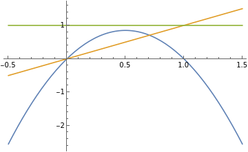
You can also solve the equation , or use FindRoot if the Solve command can't handle it.
f(x)=x
In[147]:=
a=3.4;
Solve[f[x]==x,x]
Solve[f[x]==x,x]
Out[148]=
{{x0.},{x0.705882}}
In[67]:=
a=4;Solve[f[x]==x,x]
Out[68]=
{x0},x
3
4
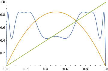
A periodic point of period is a point satisfying (p)=p, and the point is said to be of least period if (p)p for all The methods described above can also work for points of higher period. I have included an example of a search for period 3 points. To find points of period 3, we set f(f(f(x)))=x and solve for x. The Mathematica command for (x) is Nest[f,x,3]. The graph below shows the line , , and .
n
p
n
f
n
k
f
0<k<n.
3
f
y=x
y=f(x)
y=(x)
3
f
In[161]:=
a=3.4;
Plot[{Nest[f,x,4],f[x],x}, {x,0,1}, PlotRange->{0,1}]
Plot[{Nest[f,x,4],f[x],x}, {x,0,1}, PlotRange->{0,1}]
Out[162]=
We can try to solve for period 3 points using algebra, but the results aren’t great. The “Root” means that there is no way to solve for the point exactly!
In[163]:=
a=34/10.;
Solve[Nest[f,x,4]==x,x]
Solve[Nest[f,x,4]==x,x]
Out[164]=
{{x0.},{x0.0518439-0.0291111},{x0.0518439+0.0291111},{x0.170012-0.0887151},{x0.170012+0.0887151},{x0.438032-0.0595303},{x0.438032+0.0595303},{x0.451963},{x0.506526-0.199069},{x0.506526+0.199069},{x0.705882},{x0.842154},{x0.848992-0.0250849},{x0.848992+0.0250849},{x0.984592-0.0088344},{x0.984592+0.0088344}}
We can find period 2 points though.
In[75]:=
a=4;
Solve[Nest[f,x,2]==x,x]
Solve[Nest[f,x,2]==x,x]
Out[76]=
{x0},x,x(5-(5+
3
4
1
8
5
),x1
8
5
)I have included syntax and examples of each command available. To apply any command to a function not predefined in this code, define your function then put the name of your function in the command.
iterate[function, starting value, number of iterates to print, number to skip before printing]
In[153]:=
a=3.4;
iterate[f,.123,10,100]
iterate[f,.123,10,100]
Out[154]//MatrixForm=
0.842154 |
0.451963 |
0.842154 |
0.451963 |
0.842154 |
0.451963 |
0.842154 |
0.451963 |
0.842154 |
0.451963 |
0.842154 |
If you want to iterate the function -5, which is not predefined, define it the proceed as outlined. The commands below define the function, then iterate it 5 times, starting with and showing all output.
x
x=.5
In[83]:=
myfunction[x_]:=Cos[x]
In[84]:=
iterate[myfunction,3,10,0]
Out[84]//MatrixForm=
3. |
-0.989992 |
0.548696 |
0.853205 |
0.657572 |
0.791479 |
0.702794 |
0.763039 |
0.722739 |
0.749997 |
0.731691 |
Sometime we want to iterate exact values. Don't use this command unless you know that's what you want to do.
Why not use iterateexact all the time? Note that if we left the input as 0.12 Mathematica would use decimal approximations.
The next few commands are only for real functions where graphing in the plane makes sense.
This shows the iterates of a function as a graph. The iterate number is on the horizontal, and the function value is on the vertical.
This shows the iterates of a function as a graph. The iterate number is on the horizontal, and the function value is on the vertical.
Cobwebs[ function, lower limit, upper limit, starting value, number of iterates]
In[98]:=
a=3.5;
cobwebs[f,0,1,.75,10]
cobwebs[f,0,1,.75,10]
orbitwebs[function, lower limit, upper limit, starting value, number of iterates, number of iterates to skip before plotting]
In[100]:=
a=3.5;
orbitwebs[f,0,1,.734,100,20,AspectRatio->Automatic]
orbitwebs[f,0,1,.734,100,20,AspectRatio->Automatic]
Be wary of the next command - there are tolerances involved which can cause this command to give false results. It must be used with caution, but used with other commands, can be very helpful. It finds an attracting cycle if one exists.
cyclefinder[function, starting point, number of iterates to try]
In[102]:=
a=3.3;
cyclefinder[f,.123,5000]
cyclefinder[f,.123,5000]
In[104]:=
a=3.83;
cyclefinder[f,.123,5000]
cyclefinder[f,.123,5000]
In[106]:=
a=4;
cyclefinder[f,.123,5000]
cyclefinder[f,.123,5000]
We won’t be doing any of the below, but I left the pretty pictures.
Section 5.5
Section 5.5
Brief Lesson for Discrete Structures
Brief Lesson for Discrete Structures
You will may want to iterate some functions, and this file gives you a few commands to work with.