Investigating the weak censorship hypothesis in the Wolfram Model
by Nikola Bukowiecka
Space Research Centre - Polish Academy of Sciences
by Nikola Bukowiecka
Space Research Centre - Polish Academy of Sciences
This project focuses on the weak censorship hypothesis investigation in the Wolfram Model. The algorithms for calculating future null infinity, event horizons, singularities and their neighbourhood are created. The weak censorship hypothesis (presence of naked singularities) is tested in three different approaches. First, the empirical investigation of simple non-perturbed, non-trivial signature rules created spacetime. Second, the non perturbed Schwarzschild spacetime created from sprinkling. Third, the Schwarzschild spacetime created from sprinkling with Maxwell demon like spacetime perturbations introduced. Lastly, the final conclusions are formulated and the possible next steps discussed. This project investigates how common naked singularities are in the Wolfram Model and also how robust the weak cosmic censorship hypothesis is in discrete models of spacetime - especially in the Wolfram Model.
General relativity, Einstein’s equations and metric
General relativity, Einstein’s equations and metric
General relativity, being Einstein’s relativistic theory of gravity is based on three major principles the principle of equivalence , the principle of covariance and the principle of consistency.
In the Newtonian limit, general relativity predicts that the Newtonian gravitational potential approximate description of gravitation. In that sense, general relativity is consistent with the predictions of Newtonian gravitation and also with the special relativity (locally).
We define energy-momentum tensor that describes the distribution and flow of energy and momentum in a region of spacetime. Every component is a function of spacetime coordinates that describes each event in the sense of local density (with mass-energy contribution), the rate of flow of energy per unit area at right angles to the i-direction, divided by c, or, equivalently, the density of the i-component of momentum, multiplied by c, and the rate of flow of the i-component of momentum per unit area at right angles to the j-direction. This tensor is a rank 2, it’s symmetric and has ten independent components.
In order formulate the geometric theory of gravity, Einstein needed to find a geometric object that relates to the energy-momentum tensor. To do so, contractions of the Riemann curvature tensor were introduced, which allowed for the formulation of the Riemann tensor for a four- dimensional spacetime. With the vanishing of all components of the Riemann tensor one obtains a flat spacetime.
By contracting the first and last indices (which still makes the Ricci tensor symmetric with respect to interchanging its indices of the Riemann tensor, one gets a new rank 2 tensor - the Ricci tensor. Further contraction of the indicies gives the curvature scalar - the Ricci scalar.
All of these curvature-related quantities are ultimately expressed in terms of the components of the metric tensor and their derivatives. The basic ingredient of general relativity defined in terms of the Ricci tensor, the Ricci scalar and metric tensor is called the Einstein tensor.
10 of its components will be independent, just like the energy–momentum tensor. Moreover, it can be shown that the covariant divergence of the Einstein tensor vanishes, again just like the energy–momentum tensor.
The energy–momentum tensor in an important quantity for describing the ‘sources’ of gravitation, and finding another symmetric rank 2 tensor, the Einstein tensor, containing derivatives of the metric coefficients. Both the energy–momentum tensor and the Einstein tensor have zero covariant divergence, so it is natural to suggest that the two tensors are proportional. This led Einstein to propose what are now called the Einstein field equations [1].
Solving the Einstein field equations means finding the metric tensor that corresponds to a given energy–momentum tensor. Once this has been done, the geodesic equations can be used to determine the geodesics of the spacetime. These may be time-like (tangent vector always has positive norm) , space-like (the tangent vector always has negative norm) or null/light-like (the tangent vector always has zero norm).
According to the principle of geodesic motion, in general relativity the time-like geodesics of a spacetime represent the possible world-lines of massive particles falling freely under the influence of gravity alone. And, similarly, the null geodesics of a spacetime represent the possible world-lines of massless particles moving under the influence of gravity alone [1].
The Schwarzschild solutions and singularities
The Schwarzschild solutions and singularities
The Schwarzschild solution and the Schwarzschild metric
The Schwarzschild solution and the Schwarzschild metric
The ‘exterior’ Schwarzschild solution describes the spacetime geometry in the empty region surrounding a non-rotating, spherically symmetric body of mass M. In the case of the Schwarzschild solution, the relevant energy–momentum tensor is 0 since one is dealing with the empty region outside the mass distribution [1].
The particular case of the Schwarzschild solution, thanks to the spherical symmetry, the lack of time-dependence and the judicious choice of coordinates, only four of the components turn out to be non-zero, and none of them depends on x0. The solution can be represented by the diagonal matrix - the Schwarzschild metric tensor
although it is more often applied as the corresponding line element [1].
To summarize, the Schwarzschild metric is a static (and therefore stationary), spherically symmetric (invariant under rotations about the origin) solution of the Einstein field equations in the empty region exterior to any distribution of energy and momentum characterized by mass M that produces purely isotropic effects in that region. The solution is asymptotically flat, approaching the Minkowski metric in spherical coordinates for sufficiently large values of r. The solution has a coordinate singularity at the Schwarzschild radius and a gravitational singularity at r = 0, though neither of these singularities is within the region described by the solution for normal ‘star-like’ bodies [1].
Schwarzschild’s black hole and an event horizon
Schwarzschild’s black hole and an event horizon
A black hole in GR is a particular region of spacetime from which neither matter nor radiation can escape, but they can fall into it (thus the term “hole”). It’s description implies the light ring around it - since photons have no mass, they can “get the closest” to the black hole, forming an event horizon. At the heart of a black hole is a singularity that may arise from the complete gravitational collapse of some mass.
In the case of the simplest kind of black hole, which is described by the Schwarzschild metric, the event horizon is located at the Schwarzschild radius and may be thought of as a sphere. A body released from rest at a large distance from a non-rotating black hole requires only a finite proper time to reach the central singularity. Nothing unusual happens at the Schwarzschild radius [1].
In Wolfram Model the terms are constructed quite similarly. A black hole would be a region where all the edges point into, creating a separated structure. It is a region that causal edges come into, but there are no edges comming out. In the causal graph this is very visible, since one can very easily observe the vertices corresponding to events that have incoming components, but no outgoing ones. Event horizon would be the border of such structure - the surrounding layer that cloaks the singularity - being the final vertex with no outgoing components. More about the event horizon in the Section “Weak cosmic censorship in the Wolfram Model”.
Those reasons are lightcones, spacetime diagrams and causal graphs are valuable tools for investigating local spacetime structure in general relativity.
Cosmic censorship conjecture
Cosmic censorship conjecture
The weak and the strong cosmic censorship hypotheses are two mathematical conjectures about the structure of gravitational singularities arising in general relativity. The conjecture states that the maximal Cauchy development of generic compact or asymptotically flat initial data is locally inextendible as a regular Lorentzian manifold. Taken in its strongest sense, the conjecture suggests locally inextendibility of the maximal Cauchy development as a continuous Lorentzian manifold [very Strong Cosmic Censorship]. This strongest version was disproven in 2018 by Mihalis Dafermos and Jonathan Luk for the Cauchy horizon of a uncharged, rotating black hole [3].
Weak cosmic censorship hypothesis
Weak cosmic censorship hypothesis
Singularities that arise in the solutions of Einstein’s equations are typically hidden within event horizons, and therefore cannot be observed from the rest of spacetime. Singularities that are not so hidden are called naked. The weak cosmic censorship hypothesis was conceived by Roger Penrose in 1969 and posits that no naked singularities exist in the universe.
The weak cosmic censorship hypothesis asserts there can be no singularity visible from future null infinity. In other words, singularities need to be hidden from an observer at infinity by the event horizon of a black hole. Mathematically, the conjecture states that, for generic initial data, the maximal Cauchy development possesses a complete future null infinity [3].
The WCC in the Wolfram model is defined in the Section “Weak cosmic censorship in the Wolfram Model”.
Future null infinity and the geometric singularity
Future null infinity and the geometric singularity
In Minkowski spacetime the interior of the future light cone is the full future light cone at including the cone itself. If a geodesic terminates after a finite affine parameter,and it’s not possible to extend the manifold to extend the geodesic,then we have a singularity. For black holes, the future timelike boundary ends on a singularity in some places. The absolute event horizon is the past null cone of the future timelike infinity [3].
The future null infinity and the singularity in the Wolfram model are precisely defined in the Section “Weak cosmic censorship in the Wolfram Model.”
The future null infinity and the singularity in the Wolfram model are precisely defined in the Section “Weak cosmic censorship in the Wolfram Model.”
Spacetime in Wolfram model
Spacetime in Wolfram model
A complete description of this model is given by Stephen Wolfram in [5]. The essential idea here is to model space as a large collection of discrete points which, on a sufficiently large scale, resembles continuous space, in much the same way as a large collection of discrete molecules resembles a continuous fluid. A geometry can then be induced on this collection of points by introducing patterns of connections between them, as defined, for instance, by a hypergraph or set system [4].
One can connect events in the Wolfram model space by constructing a norm that allows to separate updating events in such a way that they are causally related (i.e. connected by a directed path in the causal network) if and only if they are timelike- or lightlike-separated, and spacelike-separated (i.e. connected by a family of paths in the hypergraph) [6].
Points are randomly sprinkled over the Wolfram spacetime by the sprinkling function, also defined in the Wolfram Repository.
Weak cosmic censorship in the Wolfram Model
Weak cosmic censorship in the Wolfram Model
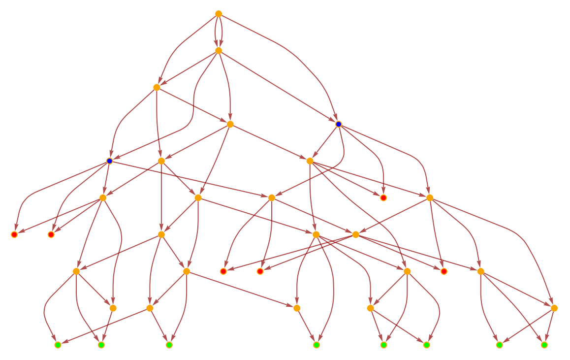
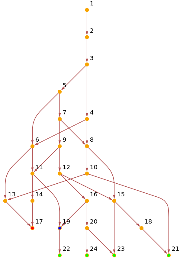
There are two important areas in which the definitions are defined that differ in the case of the empirical investigation and the sprinkled Schwarzschild space investigation.1. In the case of the empirical search: - future null infinity are verticies that have outdegree zero and are the maximal distance away from the starting starting vertex. - singularities as the vertices with the outdegree zero that are not in the future null infinity. - event horizon as the vertices that cannot reach the entire future null infinity. In the case of a relatively short computation one looks at the upper part of the causal graph to compute event horizons, because one is too low in the causal graph, the speed of life would prevent one from reaching the future infinity. In the case of infinite graphs it would not matter. - naked singularities verticies: - whose at least one of the parents (i.e casually preceding events) need to be not inside the event horizon - whose at least one of spacelike neighbours are not inside the event horizon - This actually the one that is used in this project. Space estimators are defined based on [6]. 2. In the case of the sprinkled Schwarzschild space investigation (also perturbed one): - future null infinity are the verticies with the maximal time coordinate - singularities as the vertices with the outdegree zero that are not in the future null infinity. - event horizon as the vertices that cannot reach the entire future null infinity - naked singularity - whose at least one of spacelike neighbours are not inside the EH <- I use this one. - perturbation of spacetime as drawing the edge cloaked behind the event horizon outside that region, into the non-cloaked time-like region of spacetime. To visualize the definitions in the graph below, the singularities are highlighted in red, event horizon (for example up to step 4) in blue, and the future null infinity in green.
To visualize the other definitions in the graph below, the naked singularity is highlighted in red, neighbourhood (with the space distance estimator 2) in blue, and the future null infinity in green.
The idea of the research in sprinkled spacetime is to create perturbation in spacetime that resemble Maxwell demon, which disrupts the curvature of spacetime and see if it creates any violations to the weak censorship hypothesis. Meaning to see if and how the disruptancy of the verticies behind an event horizon influence the space around it and ultimately to see if the Maxwell demon like spacetime perturbations create naked singularities which would violate the weak censorship hypothesis.
Algorithms for finding singularities in the non-trivial signature spacetime
Algorithms for finding singularities in the non-trivial signature spacetime
The section below shows step-by-step creation and investigation of the non-trivial signature spacetime expressed in terms of the causal graphs. The rule signature is {2,2} -> {2,3}. One starts with creating a set of graphs with that rule signature and the initial conditions set to {{0,0},{0,0}}. That’s the easiest non-trivial class of Wolfram Model rules.
Code execution
Code execution
Visualization of the results
Visualization of the results
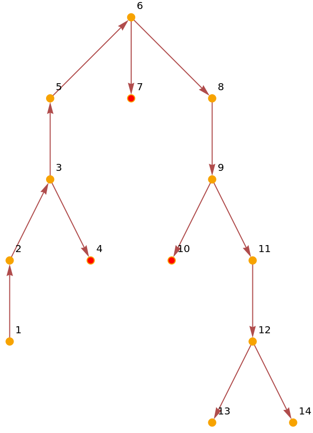
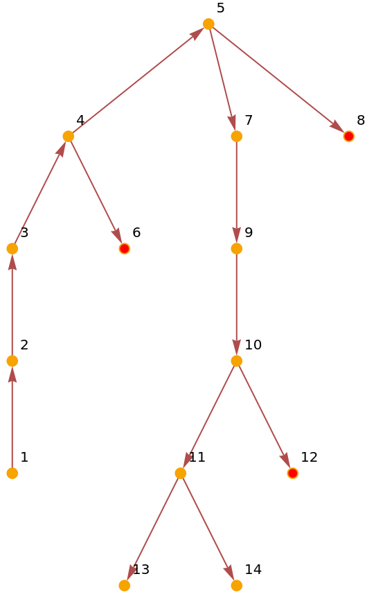
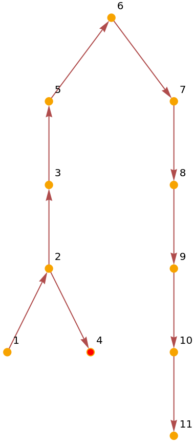
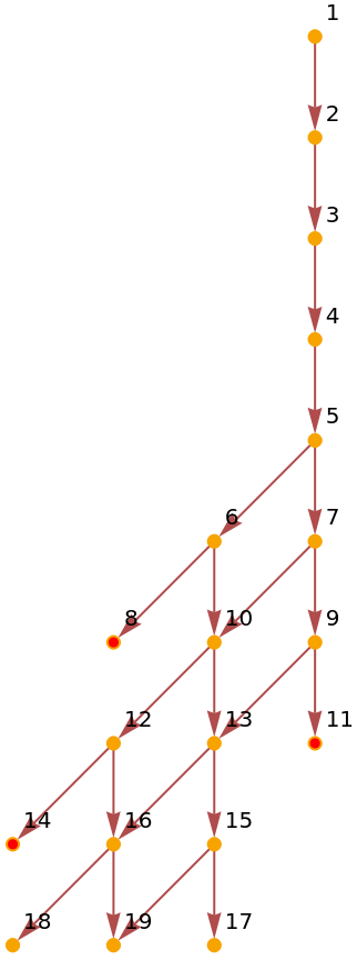
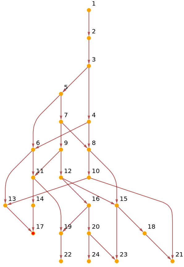
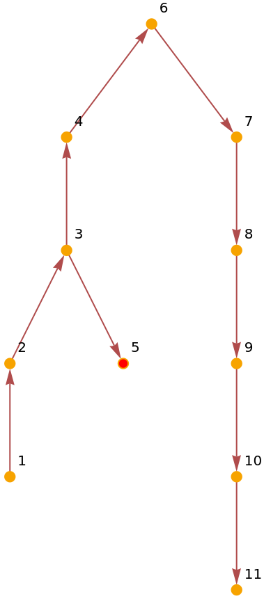
This section visualizes the graphs with naked singularities highlighted and list’s their rules.
In[]:=
visualize[evolutionLists[[graphAndSingularityNumbers[[#,1]]]][[-1]],graphAndSingularityNumbers[[#,2]]]&/@Range[Length[graphAndSingularityNumbers]]getRules[newCausalGraphList,graphAndSingularityNumbers[[#,1]]]&/@Range[Length[graphAndSingularityNumbers]]
Out[]=
,
,
,
,
,
,
Out[]=
{{{1,2},{1,3}}{{2,3},{3,4},{4,2}},{{1,2},{2,3}}{{2,2},{1,4},{3,4}},{{1,2},{1,3}}{{2,4},{3,4},{1,5}},{{1,2},{1,3}}{{4,4},{2,4},{3,2}},{{1,2},{3,2}}{{2,4},{2,1},{4,3}},{{1,2},{3,2}}{{2,4},{2,1},{4,3}},{{1,2},{3,2}}{{4,1},{1,3},{5,2}}}
Code for the specific chosen graph
Code for the specific chosen graph
Visualization for the chosen graph
Visualization for the chosen graph
Above one can find visualizations of the spatial graph and the visualizations of both neighbourhoods (blue), future null infinities (green) and singularities (red) highlighted. To see the spatial graph one needs to uncomment the code.
makeSpatialGraph[newCausalGraphList[[graphAndSingularityNumbers[[i,1]]]][[2]],{{0,0},{0,0}},10];
Spacetime with the Schwarzschild metric and a black hole
Spacetime with the Schwarzschild metric and a black hole
To simulate a 2+1 dimensional spacetime that satisfies the Schwarzschild solution with a black hole in it, one can use the code to generate random sprinkling on such spacetime or use the pre-existing example.
Checking if the singularities are behind an event horizon and visualization
Checking if the singularities are behind an event horizon and visualization
One has to check if all the verticies in the neighbourhood for a selected singularity are behind an event horizon (cannot reach entire future null infinity). In this care all the list components yield True, which mean that indeed whole neighbourhood of the selected singularity is behind an event horizon.
Visualization of the future null infinities
Visualization of the singularities
Visualization of the singularities and their neighbourhood
Perturbed spacetime with the Schwarzschild metric
Perturbed spacetime with the Schwarzschild metric
First one needs to create or load the spacetime from the section above. Then one can create random perturbations or use the example code.
Visualizations
Visualizations
Visualization consist of the graph with the two perturbations (red and green) and their out-components highlighted,
and four perturbations highlighted. Although it is not very visible, due to the fact of the over-laping of the out-components.
Resulting plot
Resulting plot
The resulting plot shows the increasing relation between the number of perturbations introduced and the ratio between the cloaked and non-cloaked events.
Concluding remarks and discussion
Concluding remarks and discussion
The increasing relation between the number of perturbations introduced and the ratio between the cloaked and non-cloaked events, means that the more perturbations we introduce, the more vertices from the singularity neighbourhood can reach future null infinity - go outside of the event horizon. This corresponds to the creation of naked singularities and violates the weak censorship hypothesis.
The important remark is that with the increase in number of points in the sprinkling, the number of fake singularities decreases - it has to do with the finite density sprinklings and the Poisson function. Fake singularities in this context mean the singularities that can be found in the “normal” spacetime, that are known not to be naked singularities. If one calculate the Minkowski space distances between the sprinkled points it’s only natural that there is non zero change of the region that is not connected with any other region. But as the number decreases with the more sprinkling points one sees that it’s not a real effect, just the effect of the functions.
The other important remark is that if we perturb the top of the light cone it does not create as many „naked singularities”/change as if we perturb from the down cone, which is theoretically predicted and has experimentally proven.
The visualizations below show how the number of “fake naked singularities” decreases with the more points sprinkled across the space.
2000 sprinkled points:
4000 sprinkled points:
6000 sprinkled points:
Summarizing, this research shows that the weak censorship hypothesis is not very robust in the discrete models of spacetime - especially in the Wolfram Model. Small perturbations influence the spacetime strongly.
Further work can will include more mathematical description of the phenomena and the extension for the strong censorship hypothesis (full cosmic censorship conjecture) by creating and analysing the energy-momenta tensor, which would fully investigate it’s validity.
Further work can will include more mathematical description of the phenomena and the extension for the strong censorship hypothesis (full cosmic censorship conjecture) by creating and analysing the energy-momenta tensor, which would fully investigate it’s validity.
Keywords
Keywords
◼
weak censorship hypothesis
◼
general relativity
◼
singularity
◼
naked singularity
◼
black hole
◼
Schwarzschild spacetime sprinkling
Acknowledgment
Acknowledgment
The projects mentor were Yorick Zeschke and Jonathan Gorard and the person who helped with the definition of the project direction was Stephen Wolfram.
References
References
◼
[1] - Robert J.A. Lambourne - Relativity, gravitation and cosmology
◼
[2] - wikipedia.org
◼
[3] - Pau Figueras, Markus Kunesch, Saran Tunyasuvunakool- End Point of Black Ring Instabilities and the Weak Cosmic Censorship Conjecture
◼
[4] - Jonathan Gorard - Some Relativistic and Gravitational Properties of the Wolfram Model
◼
[5] - S.Wolfram (2020) - A Class of Models With Potential to Represent Fundamental Physics (https: //www.wolframphysics.org/technical-introduction/)
◼
[6] - Jonathan Gorard - Algorithmic Causal Sets and the Wolfram Model