If you know how to do physics of particles and rigid bodies, how do you do physics of electromagnetic fields, quantum fields, gravitational fields? This notebook introduces a good way.
Lagrangians are black magic. They have the units of energy, and their partial derivatives yield equations of motion. Lagrangians let us solve really hard problems with minimal effort. They can be quantized and subjected to lurid geometrical and topological contortions. Pretty much all theories of physics, from classical mechanics through quantum field theory, find concise and beautiful expression through Lagrangians. Every time I write down a Lagrangian, I get excited, knowing that a solution is just around the corner.
Let me assume that you are acquainted with the Lagrangian treatment of classical particles and rigid bodies, as demonstrated in many of my notebooks to date. If not, think of Lagrangians as magical measures of energy, and you will still get something out of this notebook because you will see a familiar touchstone—Newton’s Second Law, F=ma—in several places. Other than that, I assume only knowledge of basic physics, advanced calculus, and a smattering of the Wolfram language.
In this notebook, we show how to express a classical problem, the vibrating string, in Lagrangian terms. We move
1
.from a textbook treatment with no Lagrangians
2
.to a discrete sequence of Lagrangian harmonic oscillators as particles
3
.to a limit, where there is a little bit of Lagrangian in every little bit of space
4
.to treating space and time on the same footing
5
.to a Lagrangian Density: the amount of Lagrangian per unit volume of space-time
6
.to an action, the integral of the Lagrangian density over macroscopic volumes of space-time
The Principle of Least Action (Hamilton’s Principle) yields equations of motion through the Lagrangian density. We show, here, a backwards derivation, where we get the Lagrangian density and the action by a limiting process of a sequence of Lagrangian equations of motion. We leave the forward derivation to the future.
The same ideas can take us through classical field theory and all the way through relativistic quantum field theory, where we can find expressions for the Standard Model of particle physics, for gauge theories, for the Higgs mechanism, for gravitation, and, well, everything.
This notebook is an expansion and clarification of Chapter 6 of Dwight E . Neuenschwander's Noether's Wonderful Theorem.
Notation and Quirks
Notation and Quirks
Wolfram doesn’t know how to interpret subscripted expressions like as symbols, so we write θr, etc., when we need symbols for symbolic manipulation. Wolfram also doesn’t know how to interpret overdotted expressions like as symbols, so we write qd, etc., when we need such. We could make Wolfram symbolize such expressions, but that would take us deeper into Wolfram programming than we want to go. This notebook is about physics, not about sophisticated programming.
θ
r
q
But there are a few notations you need to know.
a≡b | prose | aisDefinedAsb,orviceversa |
a≈b | prose | aisApproximatelyEqualtob |
a==b | Wolfram | AssertionofaEqualsbinWolfram |
a=b | prose | AssertionofaEqualsbinprose |
a=b | Wolfram | Assignment:"Henceforth Replace a with b" |
a->b | prose | aGoestobintheLimit |
a->b | Wolfram | RuletoReplaceExpressionawithReplacementb |
e/.r | Wolfram | ApplyReplacementRulertoExpressione |
x | prose | DifferentialofxunderanIntegral |
∂f/∂t | prose | PartialDerivativeofFunctionfbyvariablet |
D[f,t] | Wolfram | PartialDerivativeofFunctionfbyvariablet |
D[f,{t,n}] | Wolfram | nthPartialDerivative |
{...} | Wolfram | ListBracketsforGrouping |
[...] | Wolfram | BracketsEnclosingArgumentsinaFunctionCall |
We don’t need Wolfram’s total derivative, Dt, in this notebook.
Wolfram checks everything in the input-output boxes. I check my prose by hand. Trust the input-output boxes if you see a mistake in the prose.
Rule application deserves a bit of explanation. It’s the heart of the Wolfram language. The /. notation takes an expression like to its left and a rewrite rule like to its right, and rewrites the expression accordingly, e.g.,
x
{x->t}
In[]:=
x/.{x->t}
Out[]=
t
Even things that look like function calls are rule applications in disguise:
In[]:=
ClearAll[foo];foo[x_]:=x;foo[t]
Out[]=
t
Vibrating 1D String
Vibrating 1D String
The vibrating string is an elementary exercise in basic physics. It’s central to understanding stringed musical instruments like pianos, guitars, and violins. It’s analogous to vibrating 1D air columns in the wind and brass instruments. It extends to 2D drumheads and to 3D oscillators like resonant chambers.
Let’s build up the 1D problem and solve it the way one normally does in physics textbooks, no Lagrangians yet.
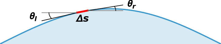
The following illustrates half a wavelength of vibrating string, with a small segment of string and two angles, ≡ (subscript little-) and ≡, tangent to the curve at the left and right ends of . The two angles are slightly different because the waveform is curved. The slopes of the tangents are slightly different at either end of .
Δs
θ
left
θ
l
l
θ
right
θ
r
Δs
Δs
The tension in the string is a force with units of mass time acceleration. It has constant magnitude but varying direction. acts along the tangent lines. The difference of the vertical components of the tensions on either side of drives the vertical motion of . In the illustrated configuration, the left angle is a little “steeper” than the right angle , so the net vertical tension force is negative, i.e., downward.
T
T
Δs
Δs
θ
l
θ
r
TSin[]-TSin[]
θ
r
θ
l
We ignore the horizontal components of the tension forces, and we ignore torque on the segment. As usual, the endpoints of the string are pinned and not allowed to move. This scenario only covers the fundamental mode of the string, where there is one half wave between the two pins.
Out[]=
Global Parameters
Global Parameters
In[]:=
ClearAll[λ];(*linearmassdensity:units*)ClearAll[T];(*tensionforcealongthestring:units*)ClearAll[Δs];(*lengthalonganelementofstring*)ClearAll[θl];(*angletotheleftofΔs[x]*)ClearAll[θr];(*angletotherightofΔs[x]*)ClearAll[v];(*horizonalspeedofthewave:units*)ClearAll[k];(*springconstant:units*)
mass
length
masslength
2
time
length
time
force
length
We already see densities peeking out: a linear mass density λ and a “force density” in the spring constant . The Lagrangian Density follows this pattern, measuring energies per unit volume of space-time. But let’s finish the textbook treatment, first.
k
Non-Linear Newtonian Equations of Motion
Non-Linear Newtonian Equations of Motion
The following is just (or, rather, ) for a small segment of string . No Lagrangians in this chapter.
F=ma
ma=F
Δs
Let the vertical displacement of a segment at time and at position be , read “phi of and .” We could call the vertical displacement , in the Cartesian (vertical) direction, but I want us to constantly remind us of a field, a quantity or value at every point in space-time, so I’ll use φ, pronounced “fie.” The field value in this problem is vertical displacement of the string, but the same idea will take us to electromagnetic fields, quantum fields for elementary particles, gauge fields, the Higgs field, the gravitational field. Same formulation, different quantities. This problem of the vibrating string really is a problem in field theory, about the easiest one I know.
Δs
t
x
φ[t,x]
t
x
y[t,x]
y
The vertical acceleration φ[t,x]≡D[φ[t,x],{t,2}] of the segment is proportional to the vertical force difference projected on the vertical axis by , at either end of the line segment. The mass of the segment is , the linear mass density λ times the length of the segment .
2
∂
∂
2
t
Sin[θ]
λΔs
Δs
(*ma=F*)λΔsD[φ[t,x],{t,2}]==T(Sin[θr[x]]-Sin[θl[x]])
Out[]=
Δsλ[t,x]T(-Sin[θl[x]]+Sin[θr[x]])
(2,0)
φ
Even this equation is approximate. It ignores the horizontal components of the forces that might stretch the string, and it ignores the torque (out of the plane) produced by the forces, which might twist the string in the plane. Those effects would only be relevant for a much more detailed or extreme scenario such as a stretchable string.
Let’s linearize , assuming small motions, so that it’s easier to solve both analytically and numerically.
ma=F
Linearized Newtonian Equations of Motion
Linearized Newtonian Equations of Motion
By small-angle approximations:
Sin[θ]≈Tan[θ]->≡D[φ[t,x],{x,1}]
∂φ[t,x]
∂x
(
1
)Δs=ΔxCos[θ]->Δx
(
2
)In[]:=
(*ma=(λΔx)φ[t,x]=F,dividingthroughbyΔx*)λD[φ[t,x],{t,2}]==T==T
2
∂
∂
2
x
(D[φ[t,x],{x,1}]/.{x->x+Δx})-(D[φ[t,x],{x,1}]/.{x->x})
Δx
ΔD[φ[t,x],{x,1}]
Δx
Out[]=
λ[t,x]
(2,0)
φ
T-[t,x]+[t,x+Δx]
(0,1)
φ
(0,1)
φ
Δx
TΔ[t,x]
(0,1)
φ
Δx
The longitudinal speed of the wave is a constant, because and λ are constants (or assumed so in this simplified version of the problem).
T
λ
T
◼
check units of as a =:
T
λ
2
speed
2
length
2
time
forceTλ==
mass
length
masslength
2
time
mass
length
2
length
2
time
Scaling by the square speed of the wave, , and recognizing the second derivative with respect to in the limit of =, we arrive at the homogeneous wave equation φ=φ:
T/λ
x
Δ∂φ/∂x
Δx
ΔD[φ[t,x],{x,1}]
Δx
2
∂
∂
2
t
2
v
2
∂
∂
2
x
In[]:=
D[φ[t,x],{t,2}]==D[φ[t,x],{x,2}]/.->
T
λ
T
λ
2
v
Out[]=
(2,0)
φ
2
v
(0,2)
φ
Analytical Solution
Analytical Solution
Following standard practice for second-order differential equations of this type, the general solution entails two arbitrary functions and .
1
2
In[]:=
ClearAll[waveEq,generalSolution];waveEq=D[φ[t,x],{t,2}]==D[φ[t,x],{x,2}];generalSolution=DSolve[waveEq,φ[t,x],{t,x}]
2
v
Out[]=
φ[t,x]-t+x+t+x
1
2
v
2
2
v
We already see time measured in units of length via the constant longitudinal speed , so that the arguments of the functions, and , check out dimensionally. This fact that time and space are commensurate when a constant velocity shows up is a central theme in relativity, which is directly implied by electromagnetic field theory. But, later for all that. For our purposes, commensurable space and time are critical to the final clean definition of Lagrangian density.
v
tv+x
-tv+x
We get a particular solution via boundary and initial conditions. We also enforce an early numerical rule that specifies a half-wave (). Without this rule, DSolve produces a more difficult expression that we don’t want to unpack.
n->1
Note the peculiar way (highlighted) we specify the initial vertical speed of the wave when one cycle is at top, at rest and about to rebound. It first calculates the symbolic partial derivative then applies a rule that replaces the symbol with the numerical value . This is idiomatic Mathematica, the Wolfram language. We abbreviate as . Six of one, half dozen of the other.
D[ϕ[t,x],t]
t->0
t
0
D[φ[t,x],{t,1}]
D[φ[t,x],t]
In[]:=
ClearAll[l,boundaryConditions,initialConditions];boundaryConditions={φ[t,0]==0,φ[t,l]==0};initialConditions=φ[0,x]==Sin,(
nπx
l
D[φ[t,x],t]/.{t->0}
)==0;A Sequence of Lagrangians
A Sequence of Lagrangians
The symmetry of space and time is shouting out! Space derivatives can be added to time derivatives with the proper scaling factors to make the units match up!
Massaging the Lagrangians
Massaging the Lagrangians
We must show how the sequence of Lagrangians yields the wave equation in the limit.
A Bit of Kinetic Energy
A Bit of Kinetic Energy
A bit of kinetic energy must be
A Bit of Potential Energy
A Bit of Potential Energy
A bit of potential energy is, as above
A Bit of Lagrangian
A Bit of Lagrangian
The terms of the wave equation, from before, shout out of this little bit of Lagrangian, ΔL. We smell the dragon nearby!
Scaling the Time Units
Scaling the Time Units
We’ll just do this by sleight-of-hand in Wolfram (manually redefining ΔL) rather than by coaxing it through Wolfram’s derivatives.
Finally, the Lagrangian Density
Finally, the Lagrangian Density
This will get us through almost everything in field-theoretical physics.
CITE THIS NOTEBOOK
CITE THIS NOTEBOOK
Backwards derivation Lagrangian density: classical 1D string segmentation bridging particle-field
by Brian Beckman
Wolfram Community, STAFF PICKS, December 1, 2025
https://community.wolfram.com/groups/-/m/t/3584475
by Brian Beckman
Wolfram Community, STAFF PICKS, December 1, 2025
https://community.wolfram.com/groups/-/m/t/3584475