In[]:=
Clear[A1,B1,C1,D1,E1,F1]
AntoineEquation=-+T
log10
sat
P
i
A
i
B
i
C
i
In[]:=
data={{60.3,70.3,80.3,90.3,100.3},{397,556,764,1031,1370}}
Out[]=
{{60.3,70.3,80.3,90.3,100.3},{397,556,764,1031,1370}}
In[]:=
DATA=Transpose[data]
Out[]=
{{60.3,397},{70.3,556},{80.3,764},{90.3,1031},{100.3,1370}}
In[]:=
Datafinal=Table[{DATA[[i]][[1]]+273.15,Log10[DATA[[i]][[2]]/760]},{i,1,5}]//N
Out[]=
{{333.45,-0.282023},{343.45,-0.135739},{353.45,0.00227977},{363.45,0.132445},{373.45,0.255907}}
In[]:=
nlm1=NonlinearModelFit[Datafinal,A1-B1/(T+C1),{A1,B1,C1},T]
Out[]=
FittedModel
In[]:=
nlm1["RSquared"]
Out[]=
1.
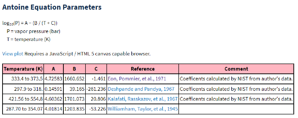
Our data agree well with coefficients obtained by NIST shown below:
In[]:=
Normal[nlm1]
Out[]=
4.719-
1659.87
-1.54355+T
ModifiedAntoineEquation=++T+ln(T)+ with=0and=2
ln
sat
P
i
A
i
B
i
C
i
D
i
E
i
F
i
T
C
i
F
i
In[]:=
Clear[A1,B1,C1,D1,E1,F1]
In[]:=
Datafinal2=Table[{DATA[[i]][[1]]+273.15,Log[DATA[[i]][[2]]/760101.325]},{i,1,5}]
Out[]=
{{333.45,3.96895},{343.45,4.30578},{353.45,4.62358},{363.45,4.9233},{373.45,5.20758}}
In[]:=
C1=0;F1=2;
In[]:=
nlm2=NonlinearModelFit[Datafinal2,A1+B1/(T+C1)+D1Log[T]+E1T^F1,{A1,B1,D1,E1},T]
Out[]=
FittedModel
In[]:=
Normal[nlm2]
Out[]=
57.2092-+8.61546×-6.53955Log[T]
5404.12
T
-6
10
2
T
In[]:=
nlm2["RSquared"]
Out[]=
1.
Clausius-ClapeyronEquation=-
ln
sat
P
i
A
i
B
i
RT
In[]:=
Clear[A1,B1,C1,D1,E1,F1]
In[]:=
data={{60.3,70.3,80.3,90.3,100.3},{397,556,764,1031,1370}}
Out[]=
{{60.3,70.3,80.3,90.3,100.3},{397,556,764,1031,1370}}
In[]:=
DATA=Transpose[data]
Out[]=
{{60.3,397},{70.3,556},{80.3,764},{90.3,1031},{100.3,1370}}
In[]:=
Datafinal=Table[{DATA[[i]][[1]]+273.15,Log[DATA[[i]][[2]]1.01325/760]},{i,1,5}]//N
Out[]=
{{333.45,-0.636219},{343.45,-0.299387},{353.45,0.0184123},{363.45,0.318129},{373.45,0.602411}}
In[]:=
R=8.314;
In[]:=
nlm3=NonlinearModelFit[Datafinal,A1-B1/(RT),{A1,B1},T]
Out[]=
FittedModel
In[]:=
3855.69×8.314
Out[]=
32056.2
In[]:=
Normal[nlm3](*Heatofvaporizationofbenzene=3855.69x8.314=32056.2kJ/kmol*)
Out[]=
10.9269-
3855.7
T
In[]:=
nlm3["RSquared"]
Out[]=
1.
Rule: The model with the lowest AIC or BIC offers the best fit.
Hence, model 1 (Antoine Equation) is better than model 2 (Modified Antoine Equation) and model 3 (Clausius-Clapeyron Equation)
Hence, model 1 (Antoine Equation) is better than model 2 (Modified Antoine Equation) and model 3 (Clausius-Clapeyron Equation)
In[]:=
nlm1["AIC"]
Out[]=
-73.9994
In[]:=
nlm1["BIC"]
Out[]=
-75.5617
In[]:=
nlm2["AIC"]
Out[]=
-63.6624
In[]:=
nlm2["BIC"]
Out[]=
-65.6152
In[]:=
nlm3["AIC"]
Out[]=
-67.5963
In[]:=
nlm3["BIC"]
Out[]=
-68.768
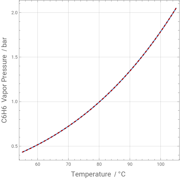
Plots of vapor pressure versus temperature show the typical exponential increasing trend
Plots of vapor pressure versus temperature show the typical exponential increasing trend
In[]:=
p1=Plot[10^(4.719-1659.87/(-1.54355+T+273.15)),{T,55,105},GridLinesAutomatic,FrameTrue,AspectRatio1,FrameLabel{Style["Temperature / °C ",14],Style["C6H6 Vapor Pressure / bar",14]}];
In[]:=
p2=Plot[Exp[57.2092-5404.12/T+8.61546*10^-6T^2-6.53955Log[T]]/101.325/.T(273.15+a),{a,55,105},GridLinesAutomatic,FrameTrue,AspectRatio1,PlotStyle{Dashed,Darker@Red}];
In[]:=
Show[p1,p2]
Out[]=
Reference
Reference
For experimental vapor pressure data versus temperature
◼
[1] C. Eon, C. Pommier, and G. Guiochon, Vapor pressures and second virial coefficients of some five-membered heterocyclic derivatives, Journal of Chemical & Engineering Data, 1971, 16 (4), pp. 408-410, DOI: 10.1021/je60051a008
CITE THIS NOTEBOOK
CITE THIS NOTEBOOK
AIC and BIC criteria for model selection applied to benzene vapor pressure versus temperature
by Housam Binous and Ahmed Bellagi
Wolfram Community, STAFF PICKS, September 15, 2024
https://community.wolfram.com/groups/-/m/t/3273909
by Housam Binous and Ahmed Bellagi
Wolfram Community, STAFF PICKS, September 15, 2024
https://community.wolfram.com/groups/-/m/t/3273909