CITE THIS NOTEBOOK: Unique father problem: Conway conjecture settled by Paul Abbott. Wolfram Community NOV 17 2022.
John Conway’s Game Of Life is endlessly fascinating. In 1972—50 years ago—Conway posed the unique father problem: Is there a stable configuration whose only father is itself?If such a configuration occurs within a universe at time , then it must have existed in the same position at time . In this note the solution found by Törmä and Salo in January 2022 is implemented and visualized.
T
T−1
Introduction
Introduction
◼
Conway’s Game Of Life, in three lines of code
◼
Several related Wolfram Demonstrations
◼
Glider Database by Ed Pegg
The (standard) Game of Life rule B3/S23 (birth/survival) is, of course, built-in. Here is the operator form of representing one step of evolution:
In[]:=
GoL=CellularAutomaton["GameOfLife"];
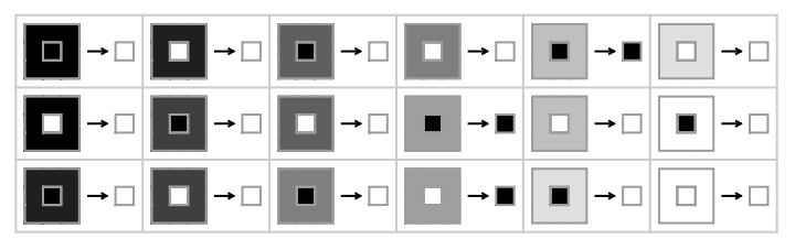
Use to examine the rule:
In[]:=
RulePlot@GoL
Out[]=
Interactive Board
Interactive Board
Start with an empty grid:
In[]:=
grid=ConstantArray[0,{15,20}];
Apply to to format the display of such grids:
In[]:=
SetOptions[ArrayPlot,{MeshTrue,MeshStyleLightGray,DataReversedTrue}];
Here is our empty grid:
In[]:=
ArrayPlot[grid]
Out[]=
Allow interactive input via mouse clicks using to define the current state:
In[]:=
state=grid;
In[]:=
n=0;
In[]:=
ClickPane[Dynamic[ArrayPlot[state]],(state=ReplacePart[state,(Reverse@Ceiling@#)1-Extract[state,Reverse@Ceiling@#]])&]
Out[]=
Compute three applications of the game of life rules:
In[]:=
ArrayPlot/@NestList[GoL,state,3]//GraphicsRow
Out[]=

Dynamically update the state and the iteration label:
In[]:=
Dynamic@ArrayPlot[state=GoL@state,PlotLabel++n]
Deleting this output stops its execution—but note that the above is still being continuously updated!
Glider
Glider
In[]:=
glider=PadLeft[{{1,1,1},{0,0,1},{0,1,0}},{20,-20}];
In[]:=
ArrayPlot@glider
Out[]=

Dynamically update the glider—and delete the output to stop execution:
Dynamic[ArrayPlot[glider=CellularAutomaton["GameOfLife"]@glider]]
Solution to the Unique Father Problem
Solution to the Unique Father Problem
An image of the (stabilised) configuration, related to the original solution found by Törmä and Salo, was published here in January:
In[]:=
img=
;
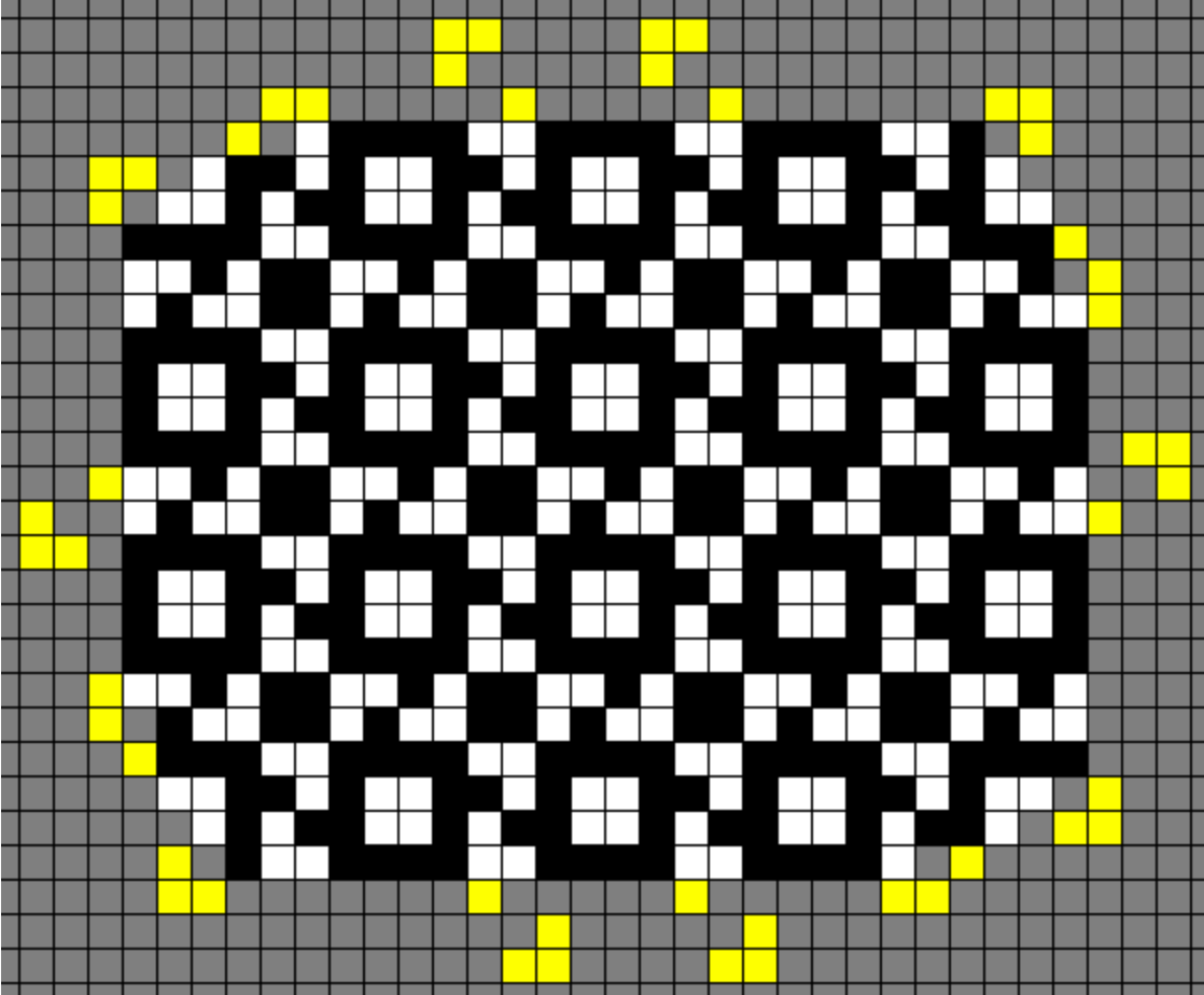
This configuration of live and dead cells is surrounded by an infinite background of grey “don't care” cells.
So, one way to investigate this solution is to use .
First Approach
First Approach
Using we can simplify the image:
In[]:=
i=ColorSeparate[img,{"Black"}][[1]]
Out[]=
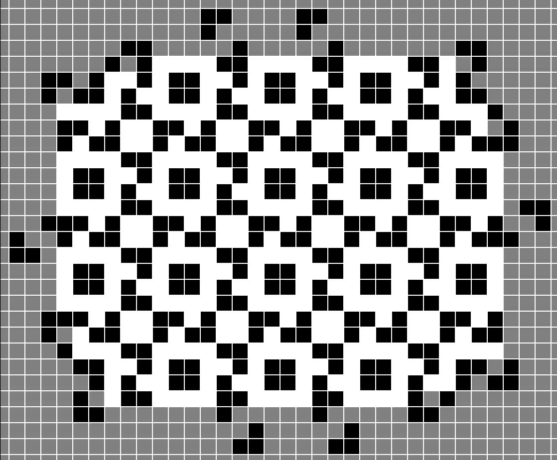
Extract the live and dead cells as follows:
As a check, apply the Game of Life rules to the stabilised configuration:
This appears to be identical. We can explicitly verify that stabilised is a solution as follows:
Second Approach
Second Approach
Markus van Almsick supplied me with the following automatic routine to detect a dark grid and to sample the brightness values in each grid cell:
Verify that stabilised2 is identical to stabilised:
Run Length Encoded Version
Run Length Encoded Version
The Run Length Encoded (or RLE for short) file format is commonly-used for storing Game of Life patterns. However, I could not find an implementation to decode this format in the Wolfram Language. But coding it up is not that hard.
From the description, the first line is a header line, which has the form
x = m, y = n
Here are replacement rules for <run_count> and <tag>:
<run_count> can be omitted if it is equal to 1—and this is also implemented as a replacement rule:
Gosper Glider Gun
Gosper Glider Gun
#N Gosper glider gun
#C This was the first gun discovered.
#C As its name suggests, it was discovered by Bill Gosper.
x = 36, y = 9, rule = B3/S23
24bo$22bobo$12b2o6b2o12b2o$11bo3bo4b2o12b2o$2o8bo5bo3b2o$2o8bo3bob2o4b
obo$10bo5bo7bo$11bo3bo$12b2o!
#C This was the first gun discovered.
#C As its name suggests, it was discovered by Bill Gosper.
x = 36, y = 9, rule = B3/S23
24bo$22bobo$12b2o6b2o12b2o$11bo3bo4b2o12b2o$2o8bo5bo3b2o$2o8bo3bob2o4b
obo$10bo5bo7bo$11bo3bo$12b2o!
Extract the RLE string:
Dynamically update the glider—and delete the output to stop execution:
Original Solution
Original Solution
x = 32, y = 26, rule = B3/S23
2 b2obo2b2obo2b2obo2b2obo2b2obo$2bob2o2bob2o2bob2o2bob2o2bob2o$2o4b2o4b
2 o4b2o4b2o4b2o$bob2o2bob2o2bob2o2bob2o2bob2o2bo$o2b2obo2b2obo2b2obo2b
2 obo2b2obo$2o4b2o4b2o4b2o4b2o4b2o$2b2obo2b2obo2b2obo2b2obo2b2obo$2bob
2 o2bob2o2bob2o2bob2o2bob2o$2o4b2o4b2o4b2o4b2o4b2o$bob2o2bob2o2bob2o2b
ob2o2bob2o2bo$o2b2obo2b2obo2b2obo2b2obo2b2obo$2o4b2o4b2o4b2o4b2o4b2o$
2 b2obo2b2obo2b2obo2b2obo2b2obo$2bob2o2bob2o2bob2o2bob2o2bob2o!
2 b2obo2b2obo2b2obo2b2obo2b2obo$2bob2o2bob2o2bob2o2bob2o2bob2o$2o4b2o4b
2 o4b2o4b2o4b2o$bob2o2bob2o2bob2o2bob2o2bob2o2bo$o2b2obo2b2obo2b2obo2b
2 obo2b2obo$2o4b2o4b2o4b2o4b2o4b2o$2b2obo2b2obo2b2obo2b2obo2b2obo$2bob
2 o2bob2o2bob2o2bob2o2bob2o$2o4b2o4b2o4b2o4b2o4b2o$bob2o2bob2o2bob2o2b
ob2o2bob2o2bo$o2b2obo2b2obo2b2obo2b2obo2b2obo$2o4b2o4b2o4b2o4b2o4b2o$
2 b2obo2b2obo2b2obo2b2obo2b2obo$2bob2o2bob2o2bob2o2bob2o2bob2o!
Extract the RLE string:
The original finite stabilisation has 374 live cells:
So the original solution looks somewhat different to the simplified solution above by Oscar Cunningham.
Verify that stable is a solution: