(I was researching this for another project, but I thought I would write up what I found here.)
There are a few different concepts which go by the name topological skeleton, but the most common is probably the medial axis. The medial axis of a region is the set of points such that every point in is equidistant to at least two points on the boundary of . It can be shown that forms a tree with the vertices of at its leaves.
R
S⊂R
S
R
S
R
Discrete
Discrete
The discrete medial axis transform is already available in Mathematica through SkeletonTransform. To demonstrate, we will first get a region for which we can generate a topological skeleton:
In[]:=
r=BoundaryDiscretizeRegionGeoGridPosition["Polygon"],"Mercator"
Out[]=
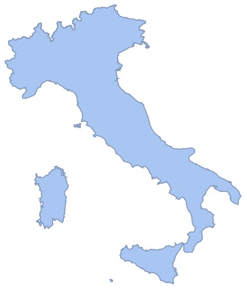
(This region has multiple connected components, but this happens to be no problem for any of the methods below.)
Then we then discretize it with Rasterize:
In[]:=
i=Rasterize[Graphics[{White,MeshPrimitives[r,2]},BackgroundBlack],RasterSize500]
Out[]=
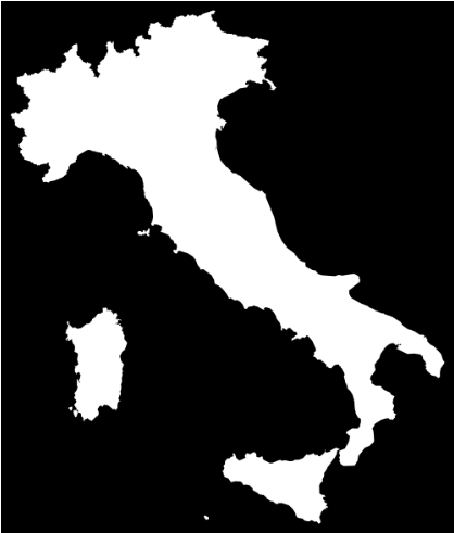
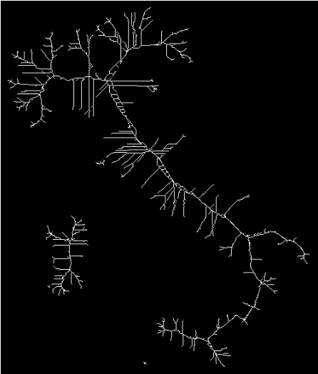
and now we can compute the skeleton transform:
In[]:=
SkeletonTransform[i]
Out[]=
and visualize it over the original (discretized) region:
In[]:=
HighlightImage[i,Binarize[SkeletonTransform[i],0]]
Out[]=
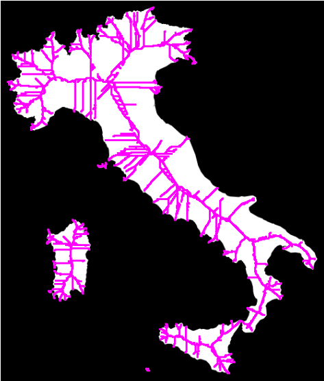
You may notice that the result is not a tree, but I think that is just a consequence of the discretization.
Continuous
Continuous
The example above works well for images (which is one of the most common uses of topological skeletons), but it does not work well for meshes, and while we might be able to use ImageMesh to approximate the continuous skeleton from the discrete one, the results are not very accurate.
Voronoi
Voronoi
The simplest way to compute the continuous medial axis is using Voronoi meshes. If we could compute Voronoi meshes with line segments, then we could compute the medial axis of every polygon exactly by finding the Voronoi mesh of every line segment on the polygon’s boundary. The edges of the resulting Voronoi mesh would correspond to points that are equidistant from two line segments on the boundary of the polygon, and therefore would be in the medial axis.
However, Voronoi meshes of line segments are more complicated than Voronoi meshes of points in part because the resulting mesh can contain curves. Mathematica does not have a builtin function for computing Voronoi diagrams of line segments, but we can get an approximate result by using many samples along the boundary:
In[]:=
vm=VoronoiMesh[MeshCoordinates[r]]
Out[]=
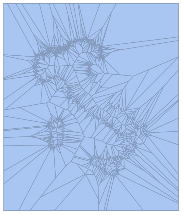
We then extract only the edges that have both endpoints in , because if an edge leads out of , then it did so between two between two vertices and is most often a consequence of out discretization of the boundary. (This leads to some problems close to the vertices of , and the result does not have the correct vertices at its leaves.)
R
R
R
In[]:=
skeleton=MeshRegion[MeshCoordinates[vm],Select[MeshCells[vm,1],ContainsOnly[Position[RegionMember[r,MeshCoordinates[vm]],True,{1},HeadsFalse][[All,1]]]@*First]]
Out[]=
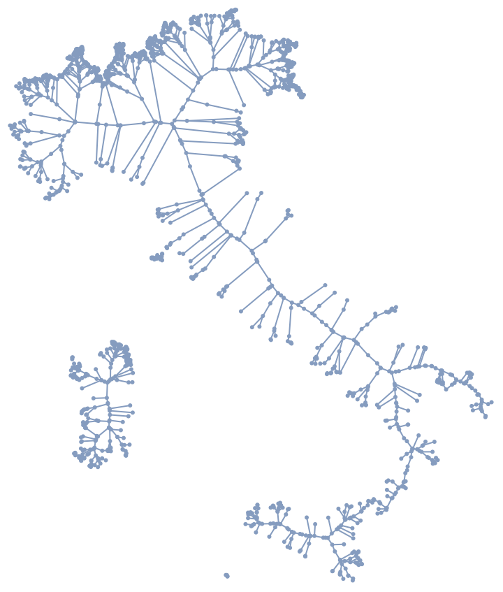
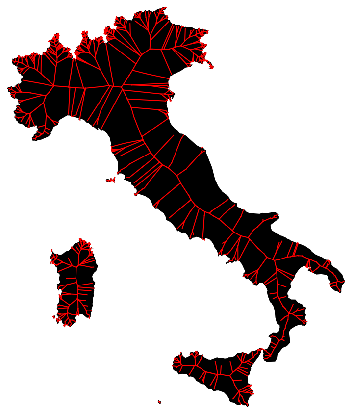
We can visualize this result on top of the original region:
In[]:=
Graphics[{MeshPrimitives[r,2],Red,MeshPrimitives[skeleton,1]}]
Out[]=
and with the Voronoi mesh:
Ridge finding
Ridge finding
I’m not sure if there is a good way to do that, but it might involve something like ContourPlot:
Construction and Motorcycle Graphs
Construction and Motorcycle Graphs
I believe this final method generates the straight skeleton and not the medial axis. Here is a good description of the algorithm:
“[T]he most readily implementable thinning algorithm starts at each vertex of the polygon and grows the skeleton inward with an edge bisecting the angle between the two neighboring edges. Eventually, these two edges meet at an internal vertex, a point equally far from three line segments. One of the three is now enclosed within a cell, while a bisector of the two surviving segments grows out from the internal vertex. This process repeats until all edges terminate in vertices.”
This seems closely related to something called a motorcycle graph which involves finding intersections of rays. However, though a inefficient implementation probably wouldn’t be too hard, getting it to run on a polygon with even 1000 points requires some algorithmic complexity.