In this project, we are analyzing cellular automata through the lens of mutation and adaptive evolution. Here, I am mutating a pre-defined integer rule multiple times to return the mutated rule that has the maximum number of cells colored the same color. I am extracting the list of rules from the integer rule, retrieving the lifetime of the automaton, and introducing a random mutation into the list of rules extracted. I am also compiling these into one main function which I am running multiple times to find the rule that works best for my code.
What is a cellular automaton?
What is a cellular automaton?
A cellular automaton is a collection of “colored” cells on a grid of a specific shape that evolves over a number of discrete time steps using a set of rules dependent on the states of neighboring cells. The rules are then applied iteratively for the specified number of time steps. It has applications across various fields like physics, biology, chemistry, computational mathematics, and computer science.
Cellular automata occur in a variety of shapes and forms. One of the most important characteristics of a cellular automaton is the grid on which it is computed. The simplest “grid” is a single-dimensional line. In two dimensions, square, triangular, and hexagonal grids can be examined. More complicated grids can also be used.
The number of colours (or distinct states) that a cellular automaton can assume must also be defined. Normally, this value is an integer, with k=2 (binary) being the most frequented and straightforward option. Colour 0 is generally referred to as “white,” and colour 1 is commonly referred to as “black” in binary automatons.
In addition to the grid and colours properties of the cellular automaton, the neighbourhood in which cells interact with one another must be described. The simplest option is “nearest neighbours,” in which only cells immediately adjacent to a specific cell are affected at each time step. In the case of a two-dimensional cellular automaton on a square grid, two frequently explored neighbourhoods are the Moore neighbourhood (square) and the von Neumann neighbourhood (diamond-shaped).
Elementary Cellular Automata
Elementary Cellular Automata
The simplest cellular automata is a one-dimensional, binary, nearest-neighbor automaton. Stephen Wolfram, who has extensively investigated their astonishing features, refers to such automata as “elementary cellular automata”. There are 256 such automata, each of which can be identified by a unique binary integer whose decimal representation is known as the “rule” for that automaton. An illustration of rule 54 is presented below, along with the evolution it creates after 30 steps beginning with a single black cell.
The rule is:
In[]:=
RulePlot[CellularAutomaton[54]]
Out[]=
The corresponding evolution is:
In[]:=
RulePlot[CellularAutomaton[54],{{1},0},30]
Out[]=
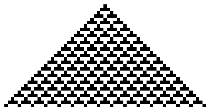
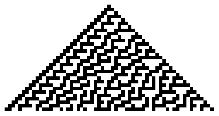
The evolution rule 54 produces is a repetitive and trivial one. Whereas, if we were to create one using rule 30 for the same number of steps, we would get a more complex pattern. This is due to rule 30 producing a chaotic evolution, the central column being given by 1, 1, 0, 1, 1, 1, 0, 0, ....
The rule is:
In[]:=
RulePlot[CellularAutomaton[30]]
Out[]=
The corresponding evolution is:
In[]:=
RulePlot[CellularAutomaton[30],{{1},0},30]
Out[]=
How cellular automata connects to evolution
How cellular automata connects to evolution
Cellular automata possess the ability to model processes that exhibit evolutionary dynamics. Simple rules in cellular automata tend to lead to complex, intricate, and unpredictable emergent patterns and behaviors, not unlike biological evolution. Natural selection and adaptability can also be simulated using cellular automata. For example, rules can be written so that some patterns (similar to organisms) have a higher survival rate dependent on their surroundings (neighboring cells). Rules may contain mechanisms for mutation and reproduction too. Cells can alter states (mutate) or influence the states of neighboring cells (reproduce), akin to genetic mutations and reproduction in biological evolution. Hence, cellular automata can be utilized to model biological evolution. This was more deeply explored by Stephen Wolfram, as witnessed in his blog post regarding this topic where he thinks of biological organisms as computational systems that follow simple rules to develop.
Aim
Aim
In this project I aim to generate rules that maximize blocks of the same color in a cellular automaton. This will be done from multiple mutations of a pre-existing rule.
Getting rule specification from integer defined rule
Getting rule specification from integer defined rule
As mentioned above, each cellular automaton is formed due to a set of rules. These rules, in Wolfram Language, are pre-compiled into integers. However, for our code, we require the entire set. Since there is no in-built function in Wolfram that can extract the set of rules from the integer for us, we need to build our own. Fortunately, the rules follow a simple pattern that we can easily duplicate by reversing the in-built function Tuples for a set range – from 0 to the number of colors -1. The function will take two arguments, the rule number itself and the number of colors we’re running the program for. Then, utilizing MapThread, we can connect the pattern we’re generating to the values we created using IntegerDigits. This code will run colors^3 times to cover all possible combinations in the pattern.
In[]:=
toCARule[ruleNumber_Integer, colors_Integer] := MapThread[#1 -> #2 &, {Reverse@Tuples[Range[0, colors - 1], 3], IntegerDigits[ruleNumber, colors, colors^3]}]
For example, to get the set of rules for four colours from rule number 160069498912288763133774917260499087900:
In[]:=
toCARule[160069498912288763133774917260499087900, 4]
Out[]=
{{3,3,3}1,{3,3,2}3,{3,3,1}2,{3,3,0}0,{3,2,3}1,{3,2,2}2,{3,2,1}3,{3,2,0}0,{3,1,3}1,{3,1,2}0,{3,1,1}0,{3,1,0}3,{3,0,3}2,{3,0,2}1,{3,0,1}3,{3,0,0}0,{2,3,3}3,{2,3,2}3,{2,3,1}1,{2,3,0}2,{2,2,3}2,{2,2,2}2,{2,2,1}2,{2,2,0}3,{2,1,3}0,{2,1,2}3,{2,1,1}1,{2,1,0}3,{2,0,3}1,{2,0,2}1,{2,0,1}2,{2,0,0}1,{1,3,3}2,{1,3,2}1,{1,3,1}2,{1,3,0}2,{1,2,3}3,{1,2,2}2,{1,2,1}0,{1,2,0}0,{1,1,3}0,{1,1,2}1,{1,1,1}0,{1,1,0}0,{1,0,3}3,{1,0,2}2,{1,0,1}2,{1,0,0}3,{0,3,3}0,{0,3,2}2,{0,3,1}2,{0,3,0}0,{0,2,3}0,{0,2,2}3,{0,2,1}0,{0,2,0}1,{0,1,3}3,{0,1,2}3,{0,1,1}0,{0,1,0}2,{0,0,3}0,{0,0,2}1,{0,0,1}3,{0,0,0}0}
This can be read in the format that when the cells follow the pattern of 3, 3, 3, the resultant cell is 1 and so on. The rule used here was taken from the blog post by Stephen Wolfram linked below in references since they are cases we know to be finite.
Getting lifetime of cellular automaton
Getting lifetime of cellular automaton
Calculating the lifespan of a cellular automaton based on its rule number and number of colors is crucial for our program. This allows us to determine when we can introduce mutation and helps us avoid potential errors in case of an infinite scenario. Since our application deals with biological evolution, the result must be finite. Therefore, an infinite lifespan is not feasible. We have developed a ‘lifeTime’ function that takes an argument list ({rule number, number of colors, radius of rule}), the number of steps after which the scenario is considered infinite, and the initial condition. The function operates on the logic that when a row of all zeros is encountered, it signifies the end of the automaton’s life. As a result, the automaton runs for a limited number of generations, and the first such row encountered is returned as the automaton’s lifespan. If such a row is not found before the specified number of steps, the function will return “NotFound,” indicating an infinite scenario.
In[]:=
lifeTime[arguments_List, steps_Integer, init_] := With[{cellAut = CellularAutomaton[arguments, init, steps]}, If[NumberQ[ FirstPosition[cellAut, ConstantArray[0, Length[cellAut[[1]]]]][[1]]], FirstPosition[cellAut, ConstantArray[0, Length[cellAut[[1]]]]][[1]], "NotFound"]]
Continuing the previous example, to get the lifetime of the cellular automaton generated by rule 160069498912288763133774917260499087900 for 4 colors:
In[]:=
lifeTime[{160069498912288763133774917260499087900, 4, 1}, 500, {{1}, 0}]
Out[]=
158
Whereas, if we consider an infinite case:
In[]:=
lifeTime[{160069412288763133774917260499087900, 4, 1}, 500, {{1}, 0}]
Out[]=
NotFound
However, this function is not completely accurate. When detecting finite cases, the lifetime returned is a little more than the actual one.
Generating random rule mutation
Generating random rule mutation
Next, to introduce mutation, we decided to change one of the values from the set of rules we extracted from the rule number earlier. Hence, taking the list as an argument, we randomly chose a key using RandomInteger from 1 to the number of choices. Upon choosing one, we changed the value of the association by replacing it with a random choice, taking measures to ensure that the same number does not get returned using RandomChoice and DeleteElements for each, respectively.
In[]:=
randomMutation[rule_List] := With[{randKey = RandomInteger[{1, Length[rule[[1]]]}]}, ReplacePart[ rule, {randKey, 2} -> RandomChoice[DeleteElements[{0, 1, 2, 3}, {rule[[randKey, 2]]}]]]]
For the same example:
In[]:=
example = toCARule[160069498912288763133774917260499087900, 4]mutatedexample = randomMutation[example]
Out[]=
{{3,3,3}1,{3,3,2}3,{3,3,1}2,{3,3,0}0,{3,2,3}1,{3,2,2}2,{3,2,1}3,{3,2,0}0,{3,1,3}1,{3,1,2}0,{3,1,1}0,{3,1,0}3,{3,0,3}2,{3,0,2}1,{3,0,1}3,{3,0,0}0,{2,3,3}3,{2,3,2}3,{2,3,1}1,{2,3,0}2,{2,2,3}2,{2,2,2}2,{2,2,1}2,{2,2,0}3,{2,1,3}0,{2,1,2}3,{2,1,1}1,{2,1,0}3,{2,0,3}1,{2,0,2}1,{2,0,1}2,{2,0,0}1,{1,3,3}2,{1,3,2}1,{1,3,1}2,{1,3,0}2,{1,2,3}3,{1,2,2}2,{1,2,1}0,{1,2,0}0,{1,1,3}0,{1,1,2}1,{1,1,1}0,{1,1,0}0,{1,0,3}3,{1,0,2}2,{1,0,1}2,{1,0,0}3,{0,3,3}0,{0,3,2}2,{0,3,1}2,{0,3,0}0,{0,2,3}0,{0,2,2}3,{0,2,1}0,{0,2,0}1,{0,1,3}3,{0,1,2}3,{0,1,1}0,{0,1,0}2,{0,0,3}0,{0,0,2}1,{0,0,1}3,{0,0,0}0}
Out[]=
{{3,3,3}1,{3,3,2}2,{3,3,1}2,{3,3,0}0,{3,2,3}1,{3,2,2}2,{3,2,1}3,{3,2,0}0,{3,1,3}1,{3,1,2}0,{3,1,1}0,{3,1,0}3,{3,0,3}2,{3,0,2}1,{3,0,1}3,{3,0,0}0,{2,3,3}3,{2,3,2}3,{2,3,1}1,{2,3,0}2,{2,2,3}2,{2,2,2}2,{2,2,1}2,{2,2,0}3,{2,1,3}0,{2,1,2}3,{2,1,1}1,{2,1,0}3,{2,0,3}1,{2,0,2}1,{2,0,1}2,{2,0,0}1,{1,3,3}2,{1,3,2}1,{1,3,1}2,{1,3,0}2,{1,2,3}3,{1,2,2}2,{1,2,1}0,{1,2,0}0,{1,1,3}0,{1,1,2}1,{1,1,1}0,{1,1,0}0,{1,0,3}3,{1,0,2}2,{1,0,1}2,{1,0,0}3,{0,3,3}0,{0,3,2}2,{0,3,1}2,{0,3,0}0,{0,2,3}0,{0,2,2}3,{0,2,1}0,{0,2,0}1,{0,1,3}3,{0,1,2}3,{0,1,1}0,{0,1,0}2,{0,0,3}0,{0,0,2}1,{0,0,1}3,{0,0,0}0}
In[]:=
SameQ[example, mutatedexample]
Out[]=
False
In the second list, we see that the value for a key is different from the value for the same key in the first. Therefore, we have successfully mutated the rule.
Maximizing a color
Maximizing a color
Ultimately, to maximize one color in the cellular automaton from multiple mutations of a pre-existing rule, we decided to compile all functions into a larger one while accounting for infinite cases simultaneously. We used the With function to encase our code. We then defined the variables steps, break, mutatedrule, and cell. steps is our call to the lifeTime function using the original rule, which is received from the argument ‘argu’ in our main function. argu is the same argument as the one we first inputted into the lifeTime function. The mutatedrule variable is a call to the pre-defined function randomMutation. The cell variable, defined for ease of reading of code, is a call to the CellularAutomaton in-built function, where it either runs till a random integer between 10 and the lifetime of the original rule or it returns nothing if the original rule generates an infinite scenario. Then, upon ensuring that the lifetime of the original rule is indeed finite, the code generates the array plot of the two joined cellular automaton: the one stored in cell and the one that follows the mutatedrule till its lifetime. For this, to ensure that the one following mutatedrule is finite, we put this in an If, where, if infinite, instead of generating an automaton, it generates the original automaton and is followed by 10 rows of a blank array. Below the array plot we print the maximum number of cells colored the same color in the mutation, excluding white.
For the same example:
Final Output
Final Output
Since we have already integrated the other functions, our final output is a call to the caColorCount function. The argument required is the same as the first one we input into the lifeTime function, i.e., the argument list, which follows the syntax {rule number, number of colors, radius of rule}. However, since we’re looking for the mutation of the rule that produces the maximum number of cells of the same color, we put the call inside a Table function that runs 10 times. This is further put inside a ReverseSortBy that sorts the generations on the basis of the last part of the output, the maximum number of cells of the same color. We then return only the first case since that is the one with the maximum number of cells of the same color in this table.
Continuing our example:
Here we see that the output comes in the form of a plot of the automaton followed by the number of cells occupied by the color most present in the automaton, i.e. blue.
Some more examples of the plots are:
For each rule here we see different mutations. Some of them do not show the latter half since the mutations in those scenarios are infinite.
Conclusion
Conclusion
Being able to find the mutated rule that causes the maximum number of cells of the same color in a table of 10 mutations of the original rule leads me to ponder its vast implications in biological evolution and cellular automata’s other applications. While fun, some parts of the code, like the caColorCount function, were not easy to code. Further, figuring out the logic behind almost every function took us time. Fortunately, in the end, we managed to complete the code and get our desired results.
Future Scope
Future Scope
Since cellular automata is an extensive concept with numerous applications across fields, there is a lot that can still be explored in it. For example, trying to achieve the same results in 2D instead of 1D can be possible, albeit tough. We tried to implement the same but it was difficult not only since we could barely find any rules for which the automaton was finite but also because there were many more minute complications that we did not have the time to consider.
Further, in 1D itself, fool proofing this code for more number of colors is also possible. These are only a few extensions that can be made to this project. However, since it is such a vast field for exploration, there can be much more done in it.
Further, in 1D itself, fool proofing this code for more number of colors is also possible. These are only a few extensions that can be made to this project. However, since it is such a vast field for exploration, there can be much more done in it.
Acknowledgements
Acknowledgements
I would like to express my sincere gratitude to my mentor, Felipe Amorim, for providing me with invaluable insights and direction throughout the duration of the Wolfram Summer Research Program. I would also like to thank our Academic Director, Eryn Gillam, for fostering a creative and comfortable environment, and always being ready to offer me advice. Further, to Nora, a teaching assistant without whom I struggled to kick off my code, I am grateful. Lastly, to the program itself, I am thankful for the opportunity to explore my interests using my pre-existing skills while learning new ones.
References
References
◼
Weisstein, Eric W. “Cellular Automaton.” From MathWorld--A Wolfram Web Resource. https://mathworld.wolfram.com/CellularAutomaton.html
◼
Weisstein, Eric W. “Elementary Cellular Automaton.” From MathWorld--A Wolfram Web Resource. https://mathworld.wolfram.com/ElementaryCellularAutomaton.html
◼
Wolfram, Stephen “Why Does Biological Evolution Work? A Minimal Model for Biological Evolution and Other Adaptive Processes,” From writings.stephenwolfram.com. https://writings.stephenwolfram.com/2024/05/why-does-biological-evolution-work-a-minimal-model-for-biological-evolution-and-other-adaptive-processes/#top.
CITE THIS NOTEBOOK
CITE THIS NOTEBOOK
Adaptive evolution of 1D cellular automata to maximize blocks of the same color
by Ahana Dalmia
Wolfram Community, STAFF PICKS, July 19, 2024
https://community.wolfram.com/groups/-/m/t/3215774
by Ahana Dalmia
Wolfram Community, STAFF PICKS, July 19, 2024
https://community.wolfram.com/groups/-/m/t/3215774