The functions sin(x) and cos(x) on its most basic form are two simple periodic waves. In this post, I explore how, from these fundamental structures, more complex ones can emerge through the application of basic transformations, such as the sum or sines or cosines and argument modifications. To introduce a greater degree of randomness, I employed irrational numbers. Using the Wolfram language an explicit visualization of the behavior can be seen, this is useful to better understand how the complex behavior are reached with a few transformations.
The simple behavior
The simple behavior
To start let’s plot the traditional and functions
sin(x)
cos(x)
In[]:=
Plot[{Sin[x],Cos[x]},{x,-2π,2π},PlotTheme->"Detailed"]
Out[]=
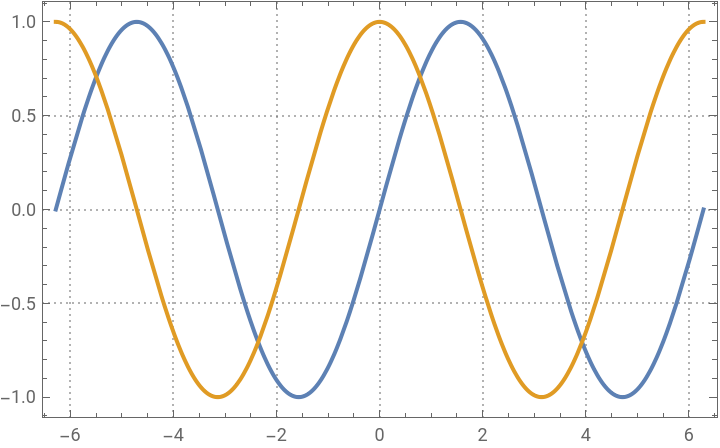


This is the phenomenon that is commonly observed, these waves are simple, there is no complexity on their behavior. Based on this simplicity a question emerges, can we get a more complex behavior from these simple functions?
This question will be addressed in the following discussion and I can tell that it is indeed possible to produce complex behaviors with these simple functions.
The modification of the argument
The modification of the argument
To start with the exploration I initially considered modifying the argument.
Here is the plot of where takes the integer values in the range
sin(αx)
α
[1,10]
In[]:=
Animate[Plot[Sin[α*x],{x,-5π,5π},PlotRange->All],{α,1,10},AnimationRunning->False]
Out[]=
Here is the plot of where takes the integer values in the range
cos(αx)
α
[1,10]
In[]:=
Animate[Plot[Cos[α*x],{x,-5π,5π},PlotRange->All],{α,1,10},AnimationRunning->False]
Out[]=
As you can see, the modification is not more complex than the original functions.
I needed to came up with more ideas, not just the modification of the parameter, and I think the following idea is the beginning of the complex behavior and an interesting discover that I did
Modify the argument and add the functions
Modify the argument and add the functions
What if, instead of just modifying the argument, we add up the functions? This shows us how the behavior changes when we do that. First we visualize the behavior of
α
∑
n1
Where α is taking the integer values in the range
[1,10]
In[]:=
Animate[Plot[Sum[Sin[n*x],{n,α}],{x,-5π,5π},PlotRange->8],{α,1,10,1},AnimationRunning->False]
Out[]=
Here we can see a more complex pattern behavior , with a series of peaks and troughs. The first spike is the largest, followed by a number of smaller waves before another big spike. It looks like if the first and last spikes are growing indefinitely, while the smaller waves are bounded. Additionally, we can see that the smaller waves are growing in both the positive and negative parts of the -axis.
y
What about the cosine function? Let’s visualize the function
Where α is taking the integer values in the range
In[]:=
Animate[Plot[Sum[Cos[n*x],{n,α}],{x,-5π,5π},PlotRange->8],{α,1,10,1},AnimationRunning->False]
Out[]=
The behavior we’re seeing is definitely more complex than what we’ve seen in the past with the function graph. Here, we can see that the big spike is bounded at the bottom but looks like it’s growing indefinitely, and the little waves are bounded.
A comparison of the behavior of the sine and cosine functions reveals a notable distinction in their respective waveforms. The sine function exhibits a symmetrical distribution of spikes, with a prominent initial wave and a comparable final wave. In contrast, the cosine function demonstrates a gradual increase in amplitude. Furthermore, the initial behavior of the two functions differs. In the sine function, the minor waves are distributed on both the positive and negative sides of the -axis. In contrast, the minor waves in the cosine function are predominantly concentrated on the negative side of the -axis.
I find it interesting to visualize it because in the plot of the section “The Simple Behavior” we can see that these functions are really alike. I was expecting a similar behavior, not some substantial difference.
Let’s visualize their behavior together
In[]:=
Animate[Plot[{Sum[Sin[n*x],{n,α}],Sum[Cos[n*x],{n,α}]},{x,-5π,5π},PlotRange->8],{α,1,10,1},AnimationRunning->False]
Out[]=
I just have focused on integer numbers as the argument, their behavior can be described as relatively simple. What if we add more randomness?
Square roots in the argument
Square roots in the argument
What if now take the past idea of adding up the functions, but rather than using integer numbers in the argument we use the square root of the number, thereby introducing greater randomness. Here we are visualizing the function
In[]:=
Animate[Plot[Sum[Sin[Sqrt[n]*x],{n,α}],{x,-5π,5π},PlotRange->All],{α,1,10},AnimationRunning->False]
Out[]=
We’re not seeing any more complex behavior here. Let’s visualize the cosine function.
When I plotted this cosine function it became evident that there were similarities in the patterns of evolution with those observed in the sine function.
What if we modify the domain, will be there some similarities?
Modifying the domain with a square root in the argument
Modifying the domain with a square root in the argument
In this section, we apply the same function as in the previous section, but with a modified domain.
It looks like the observed behavior was a local phenomenon. When the domain is modified we can see more interesting behavior. Once more, the function is grouped within the interval (20,40). It displays a distinct behavior in the vicinity of the origin and its evolution is different. What are the characteristics of the cosine function?
The functions appear to be more similar in their overall structure and behavior, exhibiting a comparable pattern around the range of 20 to 40. Let’s visualize them in the same animation to compare the behavior and get some conclusions
For me this behavior was an unexpected occurrence.The question of Whether randomness can provide a sense of order? Continues to motivate further investigation into instances where this phenomenon is observed.
Comparing the differences
Comparing the differences
CITE THIS NOTEBOOK
CITE THIS NOTEBOOK
From simple waves to complex behavior: the unpredictability of sine and cosine transformations
by Jesús Adrián Montesinos Correa
Wolfram Community, STAFF PICKS, September 18, 2024
https://community.wolfram.com/groups/-/m/t/3276382
by Jesús Adrián Montesinos Correa
Wolfram Community, STAFF PICKS, September 18, 2024
https://community.wolfram.com/groups/-/m/t/3276382