ABSTRACT (original article): We provide a complete resolution to the question of the -compactness for the solution set of the constant Q-curvature problem on a smooth closed Riemannian manifold of dimension . For dimensions , an example of an -unbounded sequence of solutions for has been known for over a decade (Wei and Zhao). On the other hand, Li and Xiong established compactness in dimensions (under some conditions). Our principal observation is that the linearized equation associated with the Q-curvature problem can be transformed into an overdetermined linear system, which admits a nontrivial solution due to an unexpected algebraic structure of the Paneitz operator. This key insight plays a crucial role in extending the compactness result to higher dimensions. CITATION (original article): Liuwei Gong, Seunghyeok Kim, Juncheng Wei (2025), Compactness of the Q-curvature problem, arXiv:2502.14237. https://doi.org/10.48550/arXiv.2502.14237
4
C
5<=n<=24
n>=25
∞
L
n>=25
5<=n<=9
One of the most important part in the paper is to verify the positivity of the matrices , , and defined in Lemmas B.11--B.13.Because it is too tedious to perform manually, we carried out these calculations using Mathematica.
D,s
m
q,
′
q
W,s
m
q,
′
q
H,s
m
q,
′
q
We start by defining several quantities. The integral Int[i,j] is the one defined in (1.4). The numbers and are defined in Proposition 6.5 or (B.16). The quantity appears in Lemma B.5 or in the proof of Lemma B.13. Finally, the number is given in the proof of Lemma B.13.
c
1
c
2
A
k,q
κ
s
Int[i_,j_]:=Integrate[t^i/(1+t^2)^j,{t,0,Infinity}]c1[n_,k_,m_]:=(k+m)(n^3-(k+m+2)n^2+(6(k+m)-4)n-4(k+m)+8);c2[n_,k_,m_]:=2(n-1)(k+m)(n+k+m-2)km;A[n_,k_,q_]:=(k-2q-1)(2-(n-2)/(n-1)*(n+k-2q-1))-(q+1)(n+2k-2q-4)kappa[n_,s_]:=(n-2)/(n-1)*s(s-1)(n+s-1)(n+s-2)
We now turn to estimating the Pohozaev quadratic form (see (6.10) for its definition). It is a bilinear form involving two symmetric 2-tensors . As shown in Corollary 6.10, the tensor can be decomposed into three mutually orthogonal components: , , and .In view of Lemma B.9, the bilinear form behaves well under this decomposition. Consequently, it suffices to examine separately in three cases, when (Case 1), (Case 2), and (Case 3).It holds that (see (6.8)) and the main order term of is , which is the content of Proposition 6.5. Moreover, 0 if or .
I
H
H
H
W
D
I
I
H=
D
H=
W
H=
H
I++
I
1
I
2
I
3
I
1
J
1
I
2
I
3
H=
D
H=
W
Case 1: Estimate of J1 with H=D
Case 1: Estimate of with
J
1
H=
D
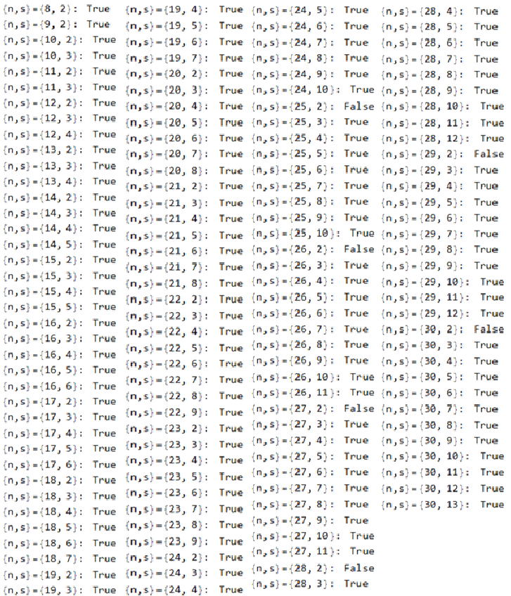
In Lemma B.11, we estimate assuming . After we define the matrix MatD ( in the paper), we simply use the Mathematica function ‘PositiveDefiniteMatrixQ’ to check its positiveness. It shows that the matrix is positive up to dimension 24. The positivity of the matrix implies the desired lower bound of in the statement of Lemma B.11.
J
1
H=
D
D,s
m
q,
′
q
J
1
Definition of the matrix
MatD[n_,s_]:=Module[{d,Msize,q,qPrime,k,m,lambdaq,lambdaqPrime,M},d=Floor[(n-4)/2];Msize=Floor[(d-s)/2]+1;M=ConstantArray[0,{Msize,Msize}];For[q=0,q<=Msize-1,q++,For[qPrime=0,qPrime<=Msize-1,qPrime++,k=2q+s;m=2qPrime+s;lambdaq=-q(n+2q+2s-2);lambdaqPrime=-qPrime(n+2qPrime+2s-2);If[k+m<n-4,M[[q+1,qPrime+1]]=1/(n-k-m-4)*Int[n+k+m-3,n-2]((8(n-1)(n-3)(k+m))/((n-2)(n+k+m-4))*lambdaq*lambdaqPrime+1/8*c1[n,k,m](2(lambdaq+lambdaqPrime)+(n+k+m-2)(k+m))-c2[n,k,m]),M[[q+1,qPrime+1]]=10^10/(2(n-3))*((8(n-1)(n-3)(k+m))/((n-2)(n+k+m-4))*lambdaq*lambdaqPrime+1/8*c1[n,k,m](2(lambdaq+lambdaqPrime)+(n+k+m-2)(k+m))-c2[n,k,m])];];];M](*//MatrixForm*)
Checking the positive definiteness
For[n=8,n<=30,n++,For[s=2,s<=Floor[(n-4)/2],s++,Print["{n,s}=",{n,s},": "PositiveDefiniteMatrixQ[MatD[n,s]]]]]
Case 2: Estimate of J1 with H=W
Case 2: Estimate of with
J
1
H=
W
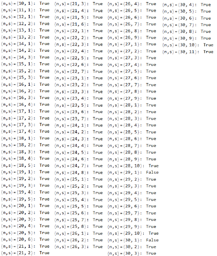
In Lemma B.12, we estimate assuming . After we define the matrix MatW ( in the paper), we simply use the Mathematica function ‘PositiveDefiniteMatrixQ’ to check its positiveness. It shows that the matrix is positive up to dimension 28. The positivity of the matrix implies the desired lower bound of in the statement of Lemma B.12.
J
1
H=
W
W,s
m
q,
′
q
J
1
Definition of the matrix
MatW[n_,s_]:=Module[{d,Msize,q,qPrime,k,m,lambdaq,lambdaqPrime,M},d=Floor[(n-4)/2];Msize=Floor[(d-s)/2];M=ConstantArray[0,{Msize,Msize}];For[q=1,q<=Msize,q++,For[qPrime=1,qPrime<=Msize,qPrime++,k=2q+s;m=2qPrime+s;lambdaq=-1/2(s+2q)(n+2q+s-2);lambdaqPrime=-1/2(s+2qPrime)(n+2qPrime+s-2);If[k+m<n-4,M[[q,qPrime]]=1/(n-k-m-4)*Int[n+k+m-3,n-2]((4(n-1)(n-3)(k+m))/((n-2)(n+k+m-4))*(4s(n+s+1)lambdaq*lambdaqPrime+kms^2(n+s)^2)+2s(n+s+1)(1/8*c1[n,k,m](2(lambdaq+lambdaqPrime)+(n+k+m-2)(k+m))-c2[n,k,m])),M[[q,qPrime]]=10^10/(2(n-3))((4(n-1)(n-3)(k+m))/((n-2)(n+k+m-4))*(4s(n+s+1)lambdaq*lambdaqPrime+kms^2(n+s)^2)+2s(n+s+1)(1/8*c1[n,k,m](2(lambdaq+lambdaqPrime)+(n+k+m-2)(k+m))-c2[n,k,m]))];];];M](*//MatrixForm*)
Checking the positive definiteness
For[n=8,n<=30,n++,For[s=1,s<=Floor[(n-4)/2]-2,s++,Print["{n,s}=",{n,s},": "PositiveDefiniteMatrixQ[MatW[n,s]]]]]
Case 3: Estimate of Iϵ with H=H
Case 3: Estimate of with
I
ϵ
H=
H
In Lemma B.13, we estimate assuming . In this case, the computation is more complicated compared to the previous cases, because we have to consider and .For this aim, we introduce further notation: The matrix and the vectors and given in Section 4.Then we define the matrices MatH1, MatH2, MatH3, and MatH (which correspond to , , , and in the proof of Lemma B.13, respectively).Then, Mathematica function ‘PositiveDefiniteMatrixQ’ yields that is positive up to dimension 32.The positivity of the matrix implies the desired lower bound of $I$ in the statement of Lemma B.13.
I
H=
H
I
2
I
3
A
b
′
b
H,s,1
m
q,
′
q
H,s,2
m
q,
′
q
H,s,3
m
q,
′
q
H,s
m
q,
′
q
H,s
m
q,
′
q
The matrix and vectors
The matrix and vectors
Definition of the matrices
Definition of the matrices
Checking the positive definiteness
CITE THIS NOTEBOOK
CITE THIS NOTEBOOK
Compactness of the Q-curvature problem
by Liuwei Gong, Seunghyeok Kim & Juncheng Wei
Wolfram Community, STAFF PICKS, May 2, 2025
https://community.wolfram.com/groups/-/m/t/3454339
by Liuwei Gong, Seunghyeok Kim & Juncheng Wei
Wolfram Community, STAFF PICKS, May 2, 2025
https://community.wolfram.com/groups/-/m/t/3454339