Diffractive optical elements (DOEs), in opposition to classical refractive optics, allow to reshape incoming radiation within very thin structure (often referred as single surface). It results not only in much lighter, compact and cost-effective structures, but also gives opportunity of obtaining light distributions unattainable by refractive approach. In order to design application specific DOE, efficient algorithms of light field propagation are necessary. So far, it has most commonly been realized with utilization of numerically calculated diffraction integrals as discrete Fourier transforms or convolutions, which is usually time and memory consuming, especially for bigger matrices.
Main goal of this project was to develop, train and verify a neural network, which emulates propagation of light in the free space and determines phase distribution of DOEs, realizing particular, as defined by the user, reshaping of incident radiation. Application of neural networks to diffractive optics allowed not only to optimize performance of the structures described by theoretical equations, but also to design DOEs realizing complex, nontrivial tasks, which couldn’t be describe with symbolic dependencies.
Main goal of this project was to develop, train and verify a neural network, which emulates propagation of light in the free space and determines phase distribution of DOEs, realizing particular, as defined by the user, reshaping of incident radiation. Application of neural networks to diffractive optics allowed not only to optimize performance of the structures described by theoretical equations, but also to design DOEs realizing complex, nontrivial tasks, which couldn’t be describe with symbolic dependencies.
Light propagation - convolution method
Light propagation - convolution method
Light can be numerically described, as a complex field of form , where A denotes amplitude of radiation and ϕ corresponds to the phase of radiation. One of the most convenient ways to describe propagation of light is based on convolving complex input field with an impulse response function (h), which in free space is defined with following equation
iϕ
Ae
h(r)=
ikz
e
iλz
2
ikr
2z
e
(
1
)where: i - imaginary number, k - wave vector, λ - wavelength, z -propagation distance.
One can simply perform this operation with utilization of built-in Wolfram Language functions. Let us define input field with gaussian amplitude and plane phase illuminating Fresnel lens with focal length equal to 100 mm.
One can simply perform this operation with utilization of built-in Wolfram Language functions. Let us define input field with gaussian amplitude and plane phase illuminating Fresnel lens with focal length equal to 100 mm.
In[]:=
lens[r_,f_,λ_]:=Exp[I*Mod[-2π/λ*Sqrt[r^2+f^2],2π]/(2π)];h[r_,z_,λ_]:=Exp[I*2π/λ*z]/(I*λ*z)*Exp[I*2π/λ/(2z)*r^2];gaussian[r_,σ_]:=Exp[-r^2/(2(σ/3)^2)];
These functions must be then properly sampled, in order to perform numerical calculations on them. Matrix and pixel size, as well as propagation constants should be provided. Then, utilizing ListConvolve, one can obtain focusing at the distance of z = 100 mm.
In[]:=
size=128;pixel=0.5;λ=0.577;σ=30;f=100;z=100;hdata=Table[h[Sqrt[x^2+y^2],100,λ],{x,-(size-1)/2*pixel,(size-1)/2*pixel,pixel},{y,-(size-1)/2*pixel,(size-1)/2*pixel,pixel}];imgdata=Table[lens[Sqrt[x^2+y^2],100,λ]*gaussian[Sqrt[x^2+y^2],σ],{x,-(size-1)/2*pixel,(size-1)/2*pixel,pixel},{y,-(size-1)/2*pixel,(size-1)/2*pixel,pixel}];con=ListConvolve[hdata,imgdata,size/2];GraphicsRow[{Image[Abs[imgdata]],Image[Arg[imgdata]],Image[(Abs[con]/Max[Abs[con]])^2],Image[(Abs[con]/Max[Abs[con]])^2]*5}]
Out[]=
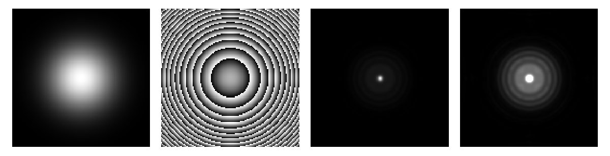
It can be seen, however, that obtained focal point is not perfect. Diffraction rings around the dot are clearly visible (right image has been multiplied by 5 to make it even more clear). In order to get rid off these patterns one has to optimize phase distribution of the designed DOE. Here, one of the first approaches of application of neural networks to this problem, is presented.
Operations on complex numbers in neural networks
Operations on complex numbers in neural networks
The first challenge was to implement operations on complex numbers into neural network framework in Wolfram Language, which currently only operates on real numbers. In order to do that, arrays of complex numbers have been described as double arrays, containing real and imaginary parts of numbers separately. Additionally, all necessary operations must also be modified to take and return real and imaginary parts separately. Layers, performing transformation of complex number form exponential to rectangular form, multiplication and convolution, are presented in subsequent paragraphs.
Exponential form
Exponential form
Layer converting complex numbers from the exponential to the rectangular form
Out[]=
NetGraph


Multiplication
Multiplication
Layer multiplying two arrays of complex numbers
Out[]=
NetGraph
Convolution
Convolution
Layer convolving the input array with the predefined kernel h
Out[]=
NetGraph
Interestingly, the complex convolution can be describe as sum of four real convolutions and it reflects calculation scheme of complex multiplication. It can be easily understood, knowing that discrete convolution is basically a sum of products.
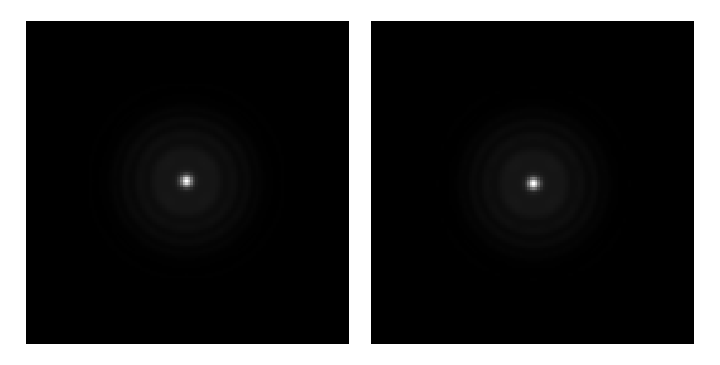
It can be easily checked, that result is the same as when using ListConvolve.
In[]:=
field={Abs[imgdata],Arg[imgdata]};conv=ConvolveComplex[field];complexConv=conv[[1]]+I*conv[[2]];GraphicsRow[{Image[Abs[complexConv]^2/Max[Abs[complexConv]^2,2]],Image[(Abs[con]/Max[Abs[con]])^2]},ImageSizeMedium]
Out[]=
Trainable net and loss functions
Trainable net and loss functions
The next step was to design a complete neural network, able firstly to perform light propagation with convolution method and secondly to calculate and optimize the phase distribution of DOE for given output amplitude distribution. The biggest issue here, was to determine proper method of calculating loss function for the purpose of neural network training. A first, not so naive, approach was to apply built-in MeanSquaredLossLayer directly to amplitude parts of output and target arrays. Controlling of the phase at the output is not necessary, as the human eye as well as commonly used detectors see only intensity of light (amplitude squared). Additional layers have been also added to implement trainable layer with phase coefficients of DOE and normalization of calculated distribution.
MeanSquaredLossLayer
MeanSquaredLossLayer
Out[]=
NetGraph

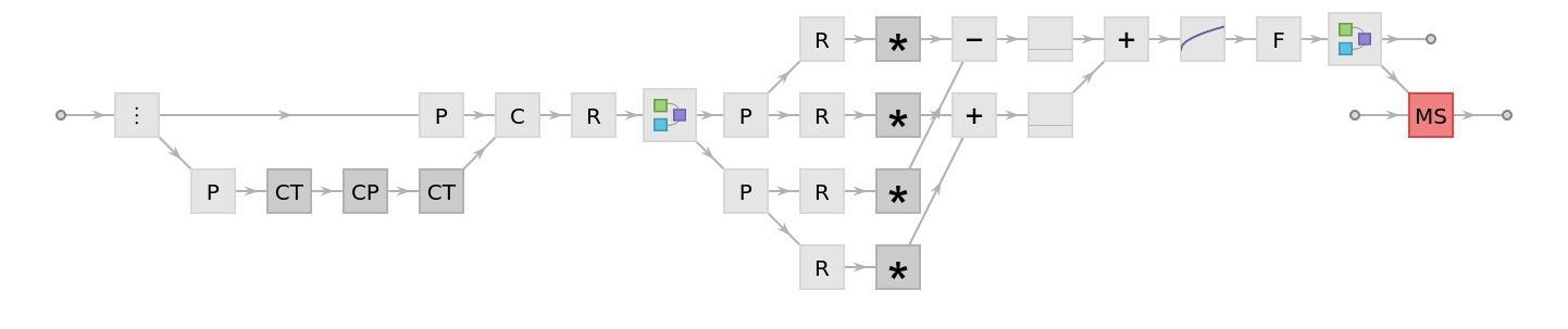

The net has been trained on the single case of light focusing, described in the previous part of this notebook. One minute of calculation time has been set as a limit, which corresponds to 13 rounds of training.

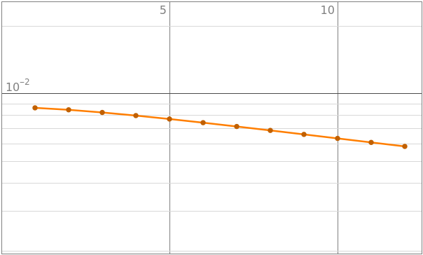
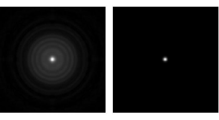
One can easily see, that the training rate is not particularly high and result is far from expected. It might be connected with the fact, that this loss function focuses on high intensity regions (central dot) and contribution from diffractive patterns with relatively lower intensity is much less significant. Given a sufficient amount of training time, it would probably be possible to obtain better results, there are however faster ways of doing that.
Alternative loss functions
Alternative loss functions
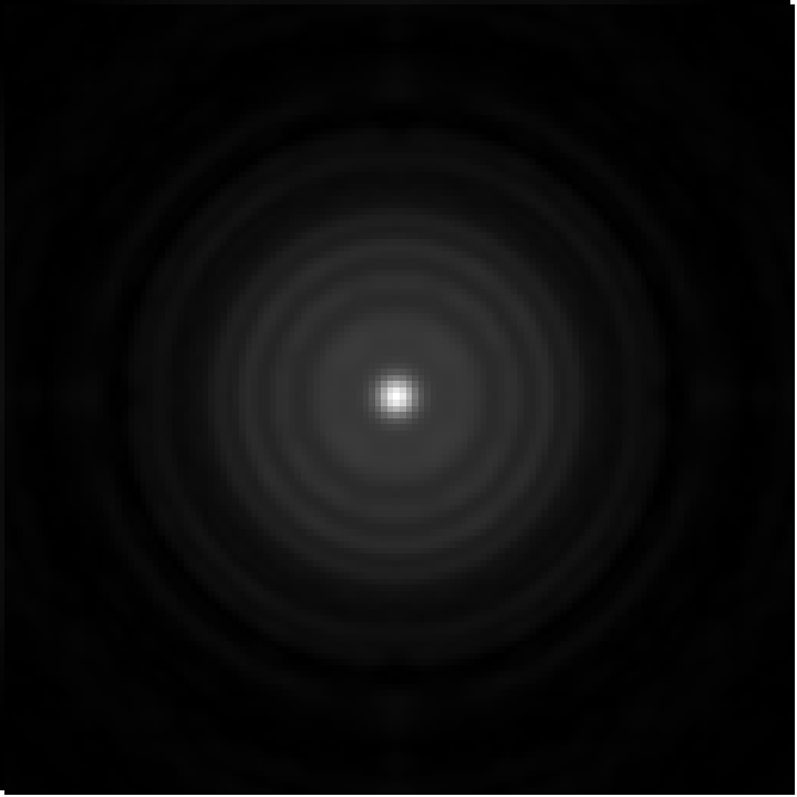
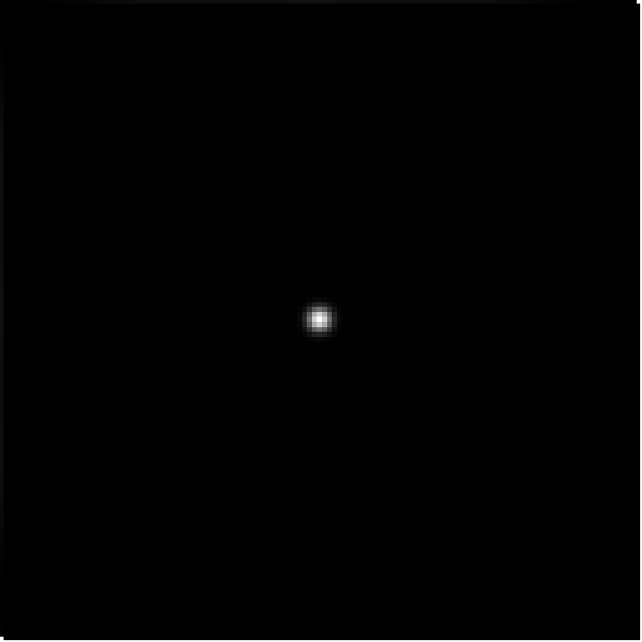
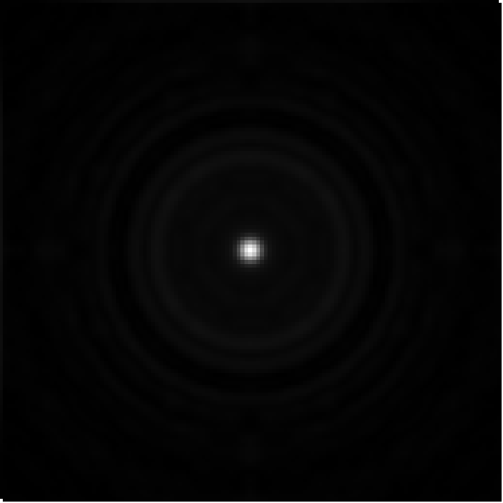
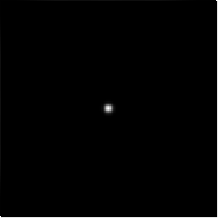
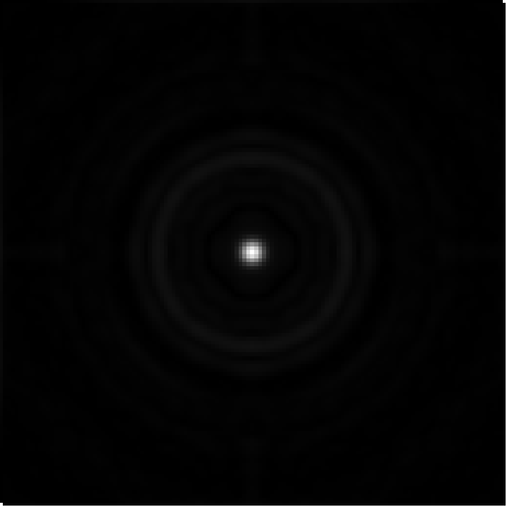
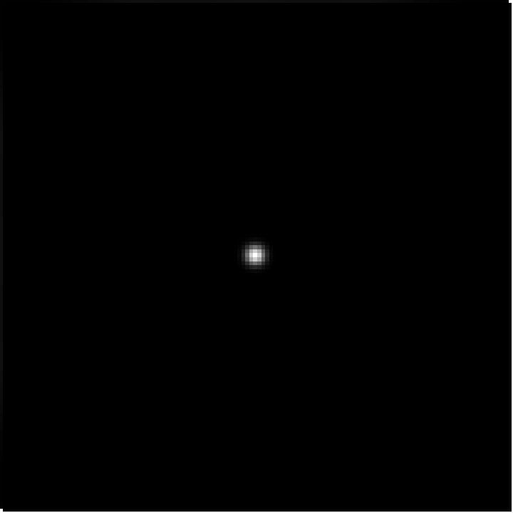
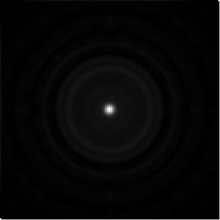
The idea was to define alternative loss functions, with enhanced impact of outer regions of the focal plane. Three approaches have been tested - difference squared, difference squared in logarithmic scale and difference quadrupled. The first one is basically manual implementation of mean squared loss, but without averaging over the image, while the other two additionally apply respectively Log and Square functions before summation. All investigated networks have been trained for the same amount of time and results have been compared with MeanSquaredLossLayer. They are shown below in an order of appearance. It can be noticed, that all proposed functions performed significantly better than MeanSquaredLossLayer (loss values smaller by an order of magnitude), while the logarithmic scale loss turned out to be the MVP with the result few times better than competitors.
In[]:=
ms=MeanSquaredLossLayer[];ms<|"Input"ImageData
[[All,All,1]],"Target"ImageData
[[All,All,1]]|>ms<|"Input"ImageData
[[All,All,1]],"Target"ImageData
[[All,All,1]]|>ms<|"Input"ImageData
[[All,All,1]],"Target"ImageData
[[All,All,1]]|>ms<|"Input"ImageData
[[All,All,1]],"Target"ImageData
[[All,All,1]]|>
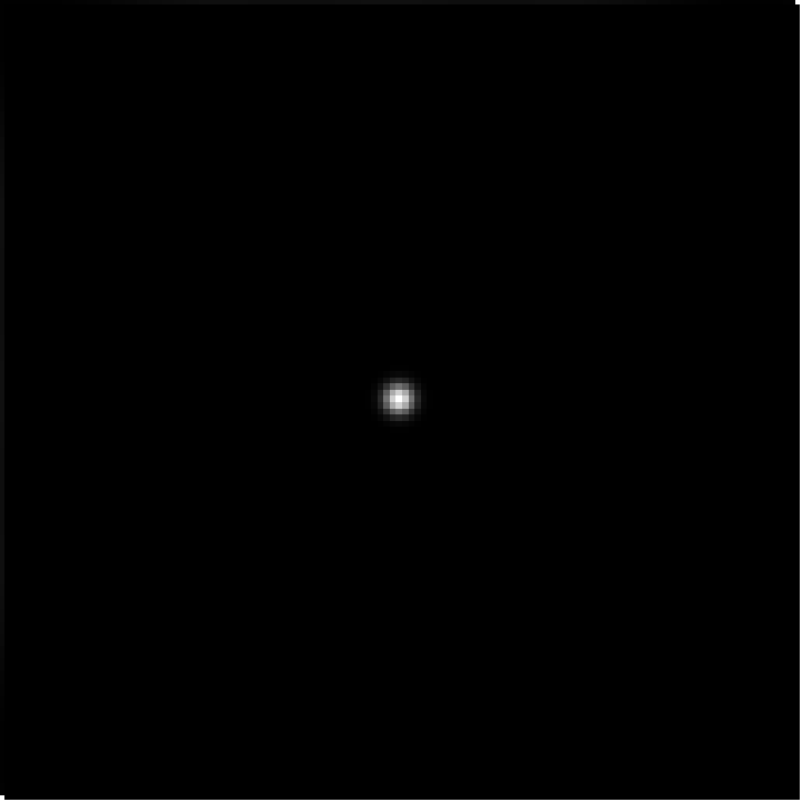
Network training for simple focusing with f = 100 mm
Network training for simple focusing with f = 100 mm
Ultimately, training of the designed net with optimized loss function can be performed.
Already after a few minutes, the value of the loss function is close to the minimum. Results of training for 1 min and 10 min are shown below, consisting of value of the loss function, output image and calculated weights (DOE). Additionally absolute minimum value of logarithmic loss function is given as a third value. It can be noticed, that after ten minutes the loss value is very close to global minimum. Interesting observations can also be made, when looking at calculated phase distributions. At the beginning it corresponds to the binary diffractive lens with alternating rings of different height, after longer training however it resembles closely Fresnel lens with smooth slopes. It is though optimized, as there are no diffractive patterns around the focal spot.
Final weights and focal spots after one and ten minutes are also shown below in the form of 3D plots.
Not only gaussian
Not only gaussian
So far, the initial amplitude was in a form of gaussian distribution. It is not the only possibility, though. Other defined or even random input fields can be tested as well. In fact, they can extend the training set, as every set of initial conditions will create a new case, although with the same target. Results of the training on the three-element set, consisting of gaussian, constant and random amplitudes as well as respective loss values are shown below. All focal points look very similar, but the value of loss function is the smallest for the gaussian amplitude. Pale diffractive patterns are visible for the latter two cases, however their shape indicates rather the square shape of aperture as origin, which is irrelevant to the amplitude distributions (in the case of gaussian amplitude, intensity in the corners of the image is very small, resulting in quasi-circular aperture).
Training time comparison
Possibilities are endless
Possibilities are endless
With all this power, why should one only calculate simple focusing cases? Much more complex, interesting and meaningful intensity distributions can be defined and the neural network will compute corresponding phase distributions (proper choice of initial conditions and learning parameters are advisable). Images below show only few of an endless number of possibilities - off-axis focusing, spikey and WSS2020 logo. From top to bottom, target image, reconstructed image and phase distribution of corresponding DOE are presented.
Conclusions
Conclusions
Propagation of light can be implemented with the tools available in the Wolfram Language. Application of neural networks allows to design and optimize various diffractive optical elements. Moreover, all presented results are not only theoretical calculations. As the wavelength and pixel size used here have been chosen on purpose to allow experimental evaluation of designed DOEs. They can easily be 3D-printed and tested in THz imaging setup, which is actually planned to be done in the foreseeable future.
Keywords
Keywords
◼
Diffractive optical elements
◼
Light propagation
◼
Neural networks
Acknowledgment
Acknowledgment
Mentor: Robert Nachbar