Changes in field ϕ over time
Changes in field ϕ over time
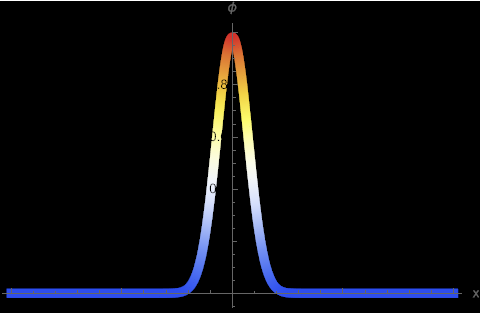
This visualization shows how the field ϕ changes over time, using a “TemperatureMap” color scheme to represent variations in the field’s amplitude.
In[]:=
c=1;m=1;hbar=1;kgEquation=D[ϕ[t,x],{t,2}]-c^2Laplacian[ϕ[t,x],{x}]+(m^2c^4)/hbar^2ϕ[t,x]==0;initialConditions={ϕ[0,x]==Exp[-x^2],Derivative[1,0][ϕ][0,x]==0};boundaryConditions={ϕ[t,-10]==0,ϕ[t,10]==0};solution=NDSolve[{kgEquation,initialConditions,boundaryConditions},ϕ,{t,0,10},{x,-10,10}];frames=Table[Plot[Evaluate[ϕ[t,x]/.solution],{x,-10,10},PlotRange->All,AxesLabel->{"x","ϕ"},ColorFunction->"TemperatureMap",ColorFunctionScaling->False,PlotStyle->Thickness[0.02],Background->Black],{t,0,10,0.1}];Export["KleinGordonAnimation.gif",frames,"DisplayDurations"->0.1]
Out[]=
KleinGordonAnimation.gif
ListAnimate[frames,AnimationRunning->False]
Out[]=
Evolution of the equation over space (x) and time (t)
Evolution of the equation over space (x) and time (t)
This code illustrates the real part of a solution to the Klein-Gordon equation as it evolves over space (x) and time (t). Run the code to see a plot that demonstrates the spatial and temporal behavior of the real component of the wavefunction, with contour lines highlighting regions of constant amplitude.
In[]:=
m=3;ω=4;ϕ[x_,t_]:=Exp[-Iωt](E^(ISqrt[ω^2-m^2]x)+E^(-ISqrt[ω^2-m^2]x));Plot3D[Re[ϕ[x,t]],{x,-5,5},{t,0,5},PlotRange->All,AxesLabel->{"Space (x)","Time (t)","Re[ϕ(x, t)]"},MeshFunctions->{#3&},MeshStyle->Opacity[0.5],BoxRatios->{1,1,1/2}]
Out[]=

Probability density | Φ (x, t) |
Probability density | Φ (x, t) |
This visualization represents the probability density |Φ(x,t)| associated with a complex superposition of plane wave solutions of the Klein-Gordon equation. We can see how this probability density evolves in space and time, with colors indicating its magnitude on a temperature map to show the behavior of the quantum field over a 2D spacetime domain.
In[]:=
m=1;ω=100;ϕ[x_,t_]:=Sum[Exp[I(kx-ωkt)]+Exp[-I(kx+ωkt)],{k,-5,5}];DensityPlot[Abs[ϕ[x,t]],{x,-5,5},{t,0,5},PlotLegends->Automatic,FrameLabel->{"Space (x)","Time (t)","|ϕ(x, t)|"},PlotRange->All,PlotPoints->100,ColorFunction->"TemperatureMap",PlotRangePadding->None]
Out[]=
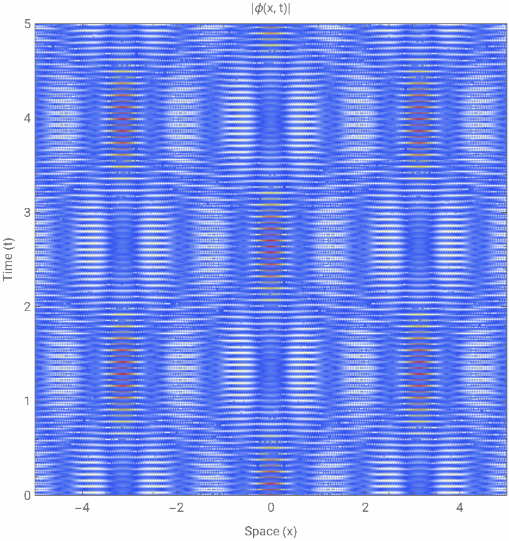

Evolution of Probability Density over space and time
Evolution of Probability Density over space and time
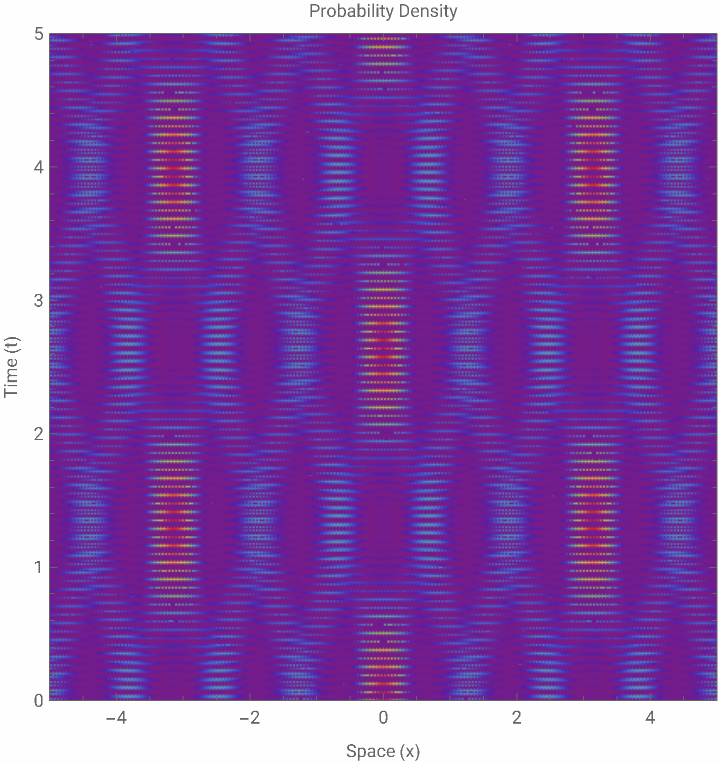
This code shows how the probability density evolves over space and time, with colors indicating the density magnitude, demonstrating the quantum behavior of the system.
In[]:=
m=1000;ω=100;ϕ[x_,t_]:=Sum[Exp[I(kx-ωkt)]+Exp[-I(kx+ωkt)],{k,-5,5}];ρ[x_,t_]:=Conjugate[ϕ[x,t]]ϕ[x,t];DensityPlot[ρ[x,t],{x,-5,5},{t,0,5},PlotLegends->Automatic,FrameLabel->{"Space (x)","Time (t)","Probability Density"},PlotRange->All,PlotPoints->100,ColorFunction->"Rainbow",PlotRangePadding->None]
Out[]=

Real and imaginary parts of a complex wavefunction
Real and imaginary parts of a complex wavefunction
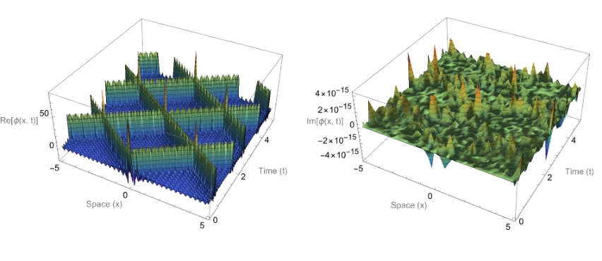
This visualization shows the real and imaginary parts of a complex wavefunction described by the Klein-Gordon equation as it evolves in space and time. The 3D plots show the spatial distribution and time evolution of the real and imaginary components of the wavefunction, with colors indicating their values.
In[]:=
m=2;ω=3;kRange=20;ϕ[x_,t_]:=Sum[Exp[I(kx-ωkt)]+Exp[-I(kx+ωkt)],{k,-kRange,kRange}];GraphicsRow[{Plot3D[Re[ϕ[x,t]],{x,-5,5},{t,0,5},PlotRange->All,AxesLabel->{"Space (x)","Time (t)","Re[ϕ(x, t)]"},MeshFunctions->{#3&},MeshStyle->Opacity[0.5],BoxRatios->{1,1,1/2},PlotPoints->50,ColorFunction->"Rainbow"],Plot3D[Im[ϕ[x,t]],{x,-5,5},{t,0,5},PlotRange->All,AxesLabel->{"Space (x)","Time (t)","Im[ϕ(x, t)]"},MeshFunctions->{#3&},MeshStyle->Opacity[0.5],BoxRatios->{1,1,1/2},PlotPoints->50,ColorFunction->"Rainbow"]}]
CITE THIS NOTEBOOK
CITE THIS NOTEBOOK
Visualizing the Klein-Gordon equation
by Dashel Myers
Wolfram Community, STAFF PICKS, September 29, 2023
https://community.wolfram.com/groups/-/m/t/3023461
by Dashel Myers
Wolfram Community, STAFF PICKS, September 29, 2023
https://community.wolfram.com/groups/-/m/t/3023461