Steady-State Temperature Distribution in Conducting Square
Steady-State Temperature Distribution in Conducting Square


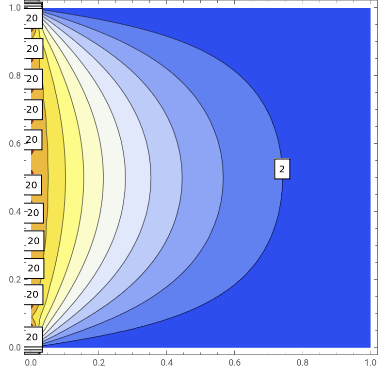
Laplace's differential equation in two dimensions, T(x,y)+T(x,y)=0, with representing a stationary temperature field, is solved in a square region. Uniform and controllable boundary conditions along the edges (excepting the corners) are considered, in a temperature range of -300 °C to 300 °C. The resulting isotherms are plotted.
2
∂
∂
2
x
2
∂
∂
2
y
T(x,y)
Details
Details
Snapshot 1: borders at 0 ºC
Snapshot 2: left border at 150 ºC and right border at -150 ºC; top and bottom are kept at 0 ºC
Snapshot 3: borders held at 150 ºC
External Links
External Links
Permanent Citation
Permanent Citation
Hernan Vivas
"Steady-State Temperature Distribution in Conducting Square"
http://demonstrations.wolfram.com/SteadyStateTemperatureDistributionInConductingSquare/
Wolfram Demonstrations Project
Published: March 7, 2011