Previous post on Hausdorff moment problem gave an analytic approach to recovering distribution from a series of moments.
This feels like “cheating” because it relies on analytic continuation.
Applying this method to a finite series of moments gives nonsensical results.
This feels like “cheating” because it relies on analytic continuation.
Applying this method to a finite series of moments gives nonsensical results.
Post below talks about:
1. inapplicability of analytic continuation
2. solving finite moment problem using non-negative least squares
3. addressing numeric stability using Chebychev polynomials
1. inapplicability of analytic continuation
2. solving finite moment problem using non-negative least squares
3. addressing numeric stability using Chebychev polynomials
Helper Utilities
Helper Utilities
Limitation of Stieltjes transform
Limitation of Stieltjes transform
To illustrate why the Stieltjes transform method fails, consider moments of the UniformDistribution
Out[]=
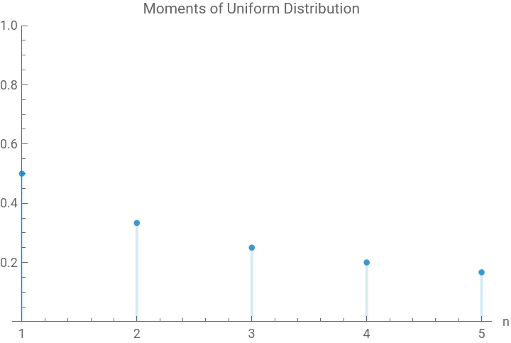


Stieltjes transform method has 3 steps:
1. take the generating function of the moment series
In[]:=
ogf=Sum,{n,0,∞}
1
1+n
n
s
Out[]=
-
Log[1-s]
s
2. Perform variable change s->1/z with a scale factor
In[]:=
stieltjes=ogf/.s
1
z
1
z
Out[]=
-Log1-
1
z
3. Visualize the imaginary part of this expression
Out[]=

Looking from the side, we can “read off” the density from the plot, that’s the essence of Stieltjes-Perron Inversion Formula (wikipedia)
Out[]=

This issue is this relies on evaluating divergent series. The value of density at x=1/2 is extracted from the value of +++... which obviously diverges
0
2
1
1
2
2
2
2
3
In[]:=
Sum/.s->2,{n,0,∞}
n
s
n+1

Out[]=
∞
∑
n=0
n
2
1+n
Switching the order of substitution invokes analytic continuation and allows Mathematica to evaluate it:
In[]:=
Sum,{n,0,∞}/.s->2
n
s
n+1
Out[]=
-
π
2
This is similar to how the value of infinite series 1+2+3+4+.... is either ∞ or -1/12 depending on whether you invoke analytic continuation
In[]:=
Print["Regular: ",Sum[/.s->-1,{k,1,∞}]];Print["Analytic continuation: ",Sum[,{k,1,∞}]/.s->-1]
-s
k
-s
k
Regular: k
∞
∑
k=1
Analytic continuation: -
1
12
Truncated Moments
Truncated Moments
Analytic continuation can’t be applied to a finite series of moments.
Instead we can setup a set of linear constraints on , .. like in this post by Daniel Lichtblau and apply LinearSolve.
However, this approach runs into issues on larger problems:
1. Basis functions like are highly correlated, so the condition number of the linear system grows exponentially, LinearSolve fails.
2. LinearSolve can produce negative probabilities, need to enforce positivity explicitly
To address this we:
1. Use non-uniform spacing for better stability
1. Make linear system optimally conditioned by applying constraints to linear combinations of moments like-3E[x]
3. Invoke QuadraticOptimization with non-negativity constraints
Instead we can setup a set of linear constraints on
E[x],E[],E[]
2
x
3
x
However, this approach runs into issues on larger problems:
1. Basis functions like
E[]
i
x
2. LinearSolve can produce negative probabilities, need to enforce positivity explicitly
To address this we:
1. Use non-uniform spacing for better stability
1. Make linear system optimally conditioned by applying constraints to linear combinations of moments like
4E[]
3
x
3. Invoke QuadraticOptimization with non-negativity constraints
We get better conditioning by packing samples more densely around 0 and 1 instead of uniform grid
In[]:=
n=100;ListPlot[{Reverse@Subdivide[.5/n,1-.5/n,n-1],.5(Cos[(Range[n]-.5)Pi/n]+1)},PlotLegends->{"Uniform grid","Chebychev"}]
Out[]=
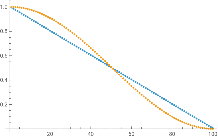

This spacing combines well with the Chebychev basis.
Compare against using the monomial basis
Compare against using the monomial basis
(E[x],E[],...,E[])
2
x
10
x
In[]:=
{n=100,m=11};xvals=.5(Cos[(Range[n]-.5)Pi/n]+1);cond[mat_]:=With[{svals=SingularValueList@mat},Max[svals]/Min[svals]];conditions=cond/@{VandermondeMatrix[xvals,m],Table[ChebyshevT[k,2p-1],{p,xvals},{k,0,m-1}]};TableForm[{conditions},TableHeadings->{{"Monomial basis","Chebychev basis"},{"condition number"}}]
Out[]//TableForm=
condition number | |
Monomial basis | 2.30635× 7 10 |
Chebychev basis | 1.41421 |
Putting this all together, recover the density of ArcSin distribution from the first 10 moments
In[]:=
ClearAll["Global`*"]{n,m}={100,11};xvals=.5(Cos[(Range[n]-.5)Pi/n]+1);yvals=PDF[ArcSinDistribution[],#]&/@xvals;{ii,zeros}={IdentityMatrix[n],ConstantArray[0,n]};A=Table[ChebyshevT[k,2p-1],{p,xvals},{k,0,m-1}];b=A.yvals;sol=QuadraticOptimization[{Transpose[A].A,-Transpose[A].b},{ii,zeros},{}];ListLinePlot[{yvals,sol},PlotLegends->{"truth","fitted"},PlotLabel->StringForm["Recovering ArcSin distribution from `` moments",m-1]]
Out[]=
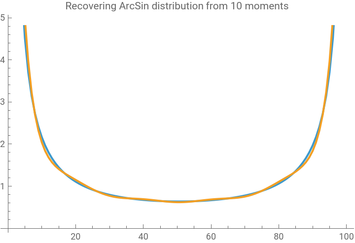


As we get more moments, error decreases
CITE THIS NOTEBOOK
CITE THIS NOTEBOOK
Hausdorff moment problem (part 2): numeric stability
by Yaroslav Bulatov
Wolfram Community, STAFF PICKS, June 21, 2025
https://community.wolfram.com/groups/-/m/t/3482655
by Yaroslav Bulatov
Wolfram Community, STAFF PICKS, June 21, 2025
https://community.wolfram.com/groups/-/m/t/3482655