Abstract (original article): Port-based teleportation (PBT) represents a variation of the standard quantum teleportation and is currently being employed and explored within the field of quantum information processing owing to its various applications. In this study, we focus on PBT protocol when the resource state is disrupted by local Pauli noises. Here, we fully characterise the channel of the noisy PBT protocol using Krauss representation. Especially, by exploiting the application of PBT for entanglement distribution necessary in realizing quantum networks, we investigate entanglement transmission through this protocol for each qubit considering noisy resource states, denoted as port-based entanglement teleportation (PBET). Finally, we derive upper and lower bounds for the teleported entanglement as a function of the initial entanglement and the noises. Our study demonstrates that quantum entanglement can be efficiently distributed by protocols utilizing large-sized resource states in the presence of noise and is expected to serve as a reliable guide for developing optimized PBET protocols. To obtain these results, we address that the order of entanglement of two qubit states is preserved through the local Pauli channel, and identify the boundaries of entanglement loss through this teleportation channel. CITATION (original article): Ha Eum Kim and Kabgyun Jeong, Port-based entanglement teleportation via noisy resource states, Phys. Scr. 99 035105 (2024). https://doi.org/10.1088/1402-4896/ad22c6
https://arxiv.org/abs/2309.01550
https://arxiv.org/abs/2309.01550
Specially in this note, we give the code to get the upper and lower bounds of entanglement reduction through the local Pauli channel as a function of average channel probabilities and initial entanglement. The main result is the last figure of this note.
Background
Background
Entanglement negativity & Pauli channel
Entanglement negativity & Pauli channel
Entanglement negativity - While von Neumann entanglement entropy captures both quantum and classical correlations in a bipartite mixed state, negativity specifically identifies quantum correlations. This characteristic also makes it a valuable tool for discerning between bipartite and multipartite quantum correlations in a pure state. Let ρ be density matrix in a multi-qudit system and be the partial transpose of the first qudit of ρ. Then if ρ is separable, all the eigenvalues of are guaranteed to be positive. In particular, for a two-qubit systems, this statement becomes not only a necessary condition to be separable, but also a sufficient condition. Therefore, the measure of entanglement for a two-qubit system can be defined by the negative eigenvalue of matrix , if it exists. This can be expressed in the form of
,
where the matrix cannot have more than one negative eigenvalue in this case.
T
1
ρ
T
1
ρ
-
λ
T
1
ρ
ℳ(ρ):=max[0,-2]
-
λ
where the matrix cannot have more than one negative eigenvalue in this case.
Pauli Channel - Pauli channel is a dominant noise source in many computing architectures generated by the system interacting with the local environment. This encompasses incoherence channel, including bit flip, bit-phase flip, phase flip, and depolarizing channel. Pauli channel at a single qubit is represented as(ρ):=;:= with >=0,where are Pauli matrix and the channel probabilities :={,,} satisfy the relation =4. Letus define one of the quantities we use to describe Pauli noise, namely the average of channel probabilities of as.
ℰ
p
3
∑
k=0
E
k
†
ρE
k
E
k
p
k
4
σ
k
p
k
σ
k
p
p
1
p
2
p
3
3
∑
k=0
p
k
ℰ
p
Ω:=
1
3
3
∑
j=1
p
j
Two-qubit entanglement reduction
Two-qubit entanglement reduction
We investigate the upper and lower bound of entanglement of bipartite pure state through local Pauli channels. Schmidt decomposition allows representing any two-qubit pure state as follows:via local unitary transformation, where . Therefore, we can express any two-qubit pure state as,where and represents Euler rotations with Euler angles :=(,,γ) and :=(,,0). The last term in is defined as zero because the z-axis rotation acting on the second qubit and the one acting on the first qubit yield the same result here. The entanglement negativity ℳ for state |ϕ⟩ is expressed as=ℳ(|ϕ〉〈ϕ|)=2sinθwhich is independent of the Euler angles.For clarity, we assume that the two qubits are far apart but interact with the same environment, resulting in the same Pauli channel acting on both qubits separately. According to this assumption, we define the entanglement of the state interacting with the environment as.
|(θ)〉:=cos|0〉⊗|0〉+sin|1〉⊗|1〉
ϕ
z
θ
2
θ
2
0<=θ<=π/2
|ϕ〉:=U()⊗V|(θ)〉
α
β
ϕ
z
U()
α
V
β
α
α
1
α
2
β
β
1
β
2
β
M
0
ℰ
p
ℳ⊗ϕϕ
ℰ
p
ℰ
p
Entanglement Reduction at Fixed Ω and θ
Entanglement Reduction at Fixed Ω and θ
This section will talk about how I got upper and lower bounds of entanglement reduction as a function of initial entanglement negativity and average channel probabilities Ω.
M
0
Step 0] Preliminary
Step 0] Preliminary
Run this cell to install Q3: https://github.com/quantum-mob/Q3. Functions named Pauli, ThePauli, TheRotation, Supermap, PartialTranspose, and Matrix are used here.
In[]:=
Module[{ps},ps=PacletSiteRegister["https://github.com/quantum-mob/PacletRepository/raw/main","Quantum Mob Paclet Server"];PacletSiteUpdate[ps];PacletInstall["Q3"]]
Out[]=
PacletObject


launch the package
In[]:=
<<Q3`
Step 1] Discretize Searching Domain
Step 1] Discretize Searching Domain
Searching in the domain of every possible entanglement reduction is impossible since variables, such as θ,, , and , are continuous. Therefore, we discretize domain for each variables. Data of the distributions of , and is uploaded at “https://github.com/HaEumKim/PBET”. Download in a folder and write down at the position where you saved at (*Insert where you saved the data*) below:
α
β
p
(,)
α
1
α
2
(,)
β
1
β
2
p
In[]:=
(*importthedata*)(*$dataU=Import["(*Insertwhereyousavedthedata*)//dataU.dat"];$dataP=Import["(*Insertwhereyousavedthedata*)//dataP.dat"];*)$dataU=Import"G:\\내 드라이브\\Research\\PBT\\data_find_boundary\\distribution\\dataU.dat";$dataP=Import"G:\\내 드라이브\\Research\\PBT\\data_find_boundary\\distribution\\dataP.dat";(*lengthforeachdata*)$Nu=Length@$dataU$Np=Length@$dataP
Out[]=
150
Out[]=
25
$dataU is used for the distribution of ) and ), while $dataP is used for the distribution of direction of . The distributions are shown as following (Activate section last section “External Codes” before activating here):
(,
α
1
α
2
(,
β
1
β
2
p
Needed definitions to produce the following graphics are found in the last section of this post.
Distribution for and
(,)
α
1
α
2
(,)
β
1
β
2
b0=Graphics3D[{Gray,Bead@BlochVector[SubEulerRotation[#].{1,0}]&/@$dataU}];Show[g1,b0,ltext,lz,ly,lx,ledge]
Out[]=
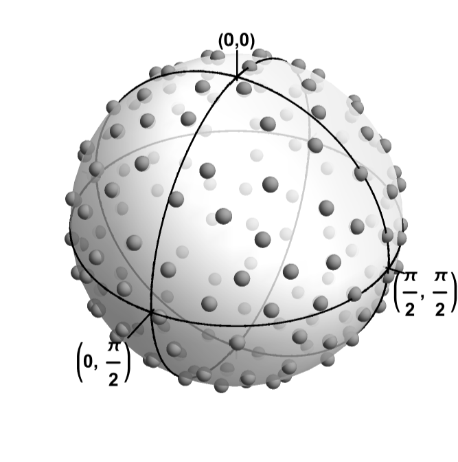
Distribution for
(,,)
p
1
p
2
p
3
lP0=Graphics3D[{Lighting->"Neutral",Gray,Sphere[#,.02]&/@$dataP}];Show[lPplane,lP0]
Out[]=

For ,
γ∈[0,4π]
Discretize γ into 2 $Nγ point, 2 π/$Nγ × {-$Nγ, -$Nγ + 1, ..., $Nγ - 1, $Nγ}
$Nγ=10;
Step 2] Search Entanglement Negativity for Specific Ω and θ
Step 2] Search Entanglement Negativity for Specific Ω and θ
We fix Ω and θ as follows:
In[]:=
$Ω=0.12013073152096207`;$θ=0.2013579207903308`;
We are ready to search entanglement negativity for the total discretized domain of two-qubit state with local Pauli channel with fixed Ω and θ.
Step 3] Analysis
Step 3] Analysis
It shows that the channel probabilities of lowest 1000 and highest 1000 entanglement negativity are near bit-flip, bit-phase flip, and phase flip.
To find the form of initial state, we select the channel as phase flip
Construct phase flip channel
Function to calculate negativity . It uses the part of the function “ListInfoMout”
The states of lower bound we found is smaller than the minimum we got numerically
The states of upper bound we found is higher than the maximum we got numerically
Defining γ for the state lower bound. γ has to be ± i
Boundary of Entanglement Negativity
Boundary of Entanglement Negativity
Even we change the average of channel probabilities Ω and angle θ of initial state, the states of lower and upper bounds doesn’t change. This can be seen by changing $Ω and $θ of the above code. Finally, we can calculate the upper and lower bound of entanglement negativity for every fixed Ω and θ by the result of states of boundaries. For details see our original article.
External Codes
External Codes
Graphics
Graphics
CITE THIS NOTEBOOK
CITE THIS NOTEBOOK
Port-based entanglement teleportation via noisy resource states
by Ha Eum Kim & Kabgyun Jeong
Wolfram Community, STAFF PICKS, November 6, 2024
https://community.wolfram.com/groups/-/m/t/3315499
by Ha Eum Kim & Kabgyun Jeong
Wolfram Community, STAFF PICKS, November 6, 2024
https://community.wolfram.com/groups/-/m/t/3315499