This problem is available at https://web.mit.edu/10.213/www/problemsets.shtml
A two-stage cascade refrigeration system employs difluoromethane (R32 or CH2F2) as refrigerant in Cycle 1 and tetrafluoroethane (R134A or C2H2F4) as refrigerant in Cycle 2.
Thermodynamic data for tetrafluoroethane and difluoromethane are found at http://webbook.nist.gov/chemistry/fluid/.
A two-stage cascade refrigeration system employs difluoromethane (R32 or CH2F2) as refrigerant in Cycle 1 and tetrafluoroethane (R134A or C2H2F4) as refrigerant in Cycle 2.
Thermodynamic data for tetrafluoroethane and difluoromethane are found at http://webbook.nist.gov/chemistry/fluid/.
Cycle 1 operates with an evaporation temperature of -55 °F and a condensation temperature of 0 °F.Cycle 2 operates with an evaporation temperature of -10 °F and a condensation temperature of 90 °F. Both cycles employ compressors with efficiencies of 75%.
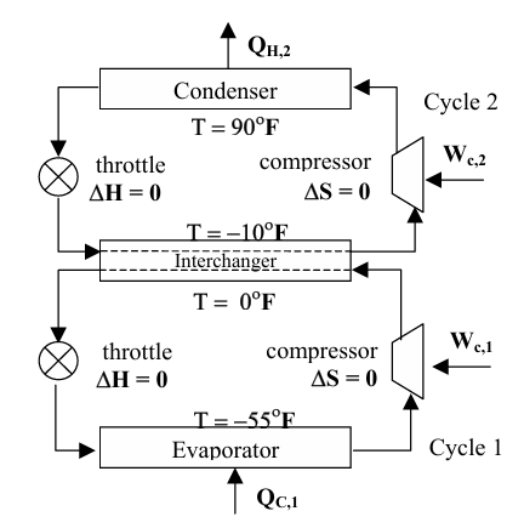
Limits on the operating pressures of the evaporator and condenser of a refrigeration system also limit the temperature difference TH − TC over which a single cycle can operate (see Ref. 1). Since TH is fixed by the temperature of the surroundings, a lower limit is placed on the temperature level of refrigeration or TC (see Ref. 1). By operating two refrigeration cycles using different refrigerants in a cascade, this limitation can be overcome. Here, the two cycles operate so that the heat absorbed in the inter-changer by the refrigerant of the higher-temperature cycle 2 serves to condense the refrigerant in the lower temperature cycle 1. Moreover, in case of a single cycle for example with R134A, the pressure ratio would be 25.22, which is too high to achieve with a single-stage compressor.
CYCLE 2
CYCLE 2
saturation properties - pressure increment = 5 psia
Temperature (F), Pressure (psia), Enthalpy (Btu/lbm), Entropy (Btu/lbm*R), Enthalpy (Btu/lbm), Entropy (Btu/lbm*R)
Temperature (F), Pressure (psia), Enthalpy (Btu/lbm), Entropy (Btu/lbm*R), Enthalpy (Btu/lbm), Entropy (Btu/lbm*R)
datasat=;
In[]:=
tblhl=Table[{datasat[[i]][[2]],datasat[[i]][[3]]},{i,1,Length[datasat]}];tblsl=Table[{datasat[[i]][[2]],datasat[[i]][[4]]},{i,1,Length[datasat]}];
In[]:=
fhl=Interpolation[tblhl];fsl=Interpolation[tblsl];
In[]:=
tblhv=Table[{datasat[[i]][[2]],datasat[[i]][[5]]},{i,1,Length[datasat]}];tblsv=Table[{datasat[[i]][[2]],datasat[[i]][[6]]},{i,1,Length[datasat]}];
In[]:=
fhv=Interpolation[tblhv];fsv=Interpolation[tblsv];
In[]:=
tbltp=Table[{datasat[[i]][[1]],datasat[[i]][[2]]},{i,1,Length[datasat]}];
In[]:=
ftp=Interpolation[tbltp];
In[]:=
ftp[90]
Out[]=
119.014
In[]:=
ftp[-10]
Out[]=
16.6318
In[]:=
pressureRATIO=ftp[90]/ftp[-10]
Out[]=
7.15583
In[]:=
pressureRATIO=ftp[90]/ftp[-55]
Out[]=
25.2284
isobaric properties - pressure = 119.014 psia
{Temperature (F), Pressure (psia), Enthalpy (Btu/lbm), Entropy (Btu/lbm*R), State)}
{Temperature (F), Pressure (psia), Enthalpy (Btu/lbm), Entropy (Btu/lbm*R), State)}
dataisobaric=;
In[]:=
pos=Position[dataisobaric,90.000]
Out[]=
{{286,1},{287,1}}
In[]:=
tblhsv=Table[{dataisobaric[[i]][[1]],dataisobaric[[i]][[3]]},{i,287,Length[dataisobaric]}];tblssv=Table[{dataisobaric[[i]][[1]],dataisobaric[[i]][[4]]},{i,287,Length[dataisobaric]}];tblshsv=Table[{dataisobaric[[i]][[4]],dataisobaric[[i]][[3]]},{i,287,Length[dataisobaric]}];
In[]:=
fshsv=Interpolation[tblshsv];
In[]:=
tblhl1=Table[{datasat[[i]][[3]],datasat[[i]][[2]]},{i,1,Length[datasat]}];tblsl1=Table[{datasat[[i]][[4]],datasat[[i]][[1]]},{i,1,Length[datasat]}];
In[]:=
tblhv1=Table[{datasat[[i]][[5]],datasat[[i]][[2]]},{i,1,Length[datasat]}];tblsv1=Table[{datasat[[i]][[6]],datasat[[i]][[1]]},{i,1,Length[datasat]}];
In[]:=
fhsv=Interpolation[tblhsv];fssv=Interpolation[tblssv];
In[]:=
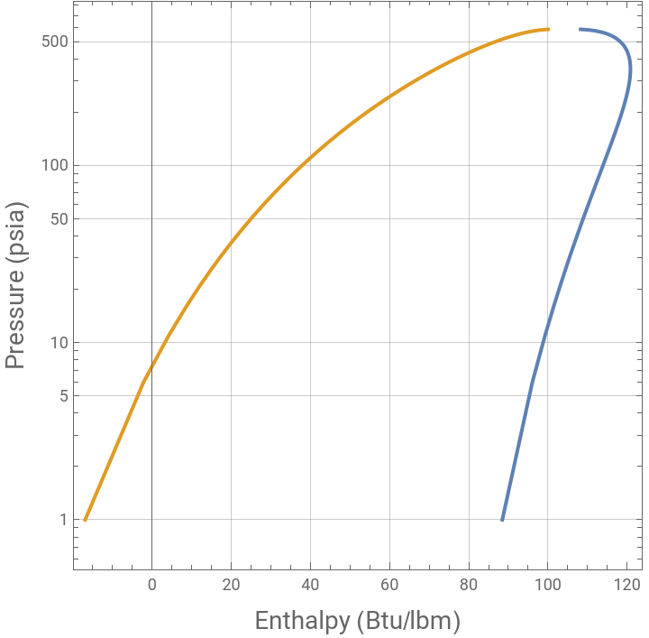
plt1=ListLogPlot[{tblhv1,tblhl1},JoinedTrue,FrameTrue,AspectRatio1,GridLinesAutomatic,FrameLabel{Style["Enthalpy (Btu/lbm)",14],Style["Pressure (psia)",14]}]
Out[]=
In[]:=
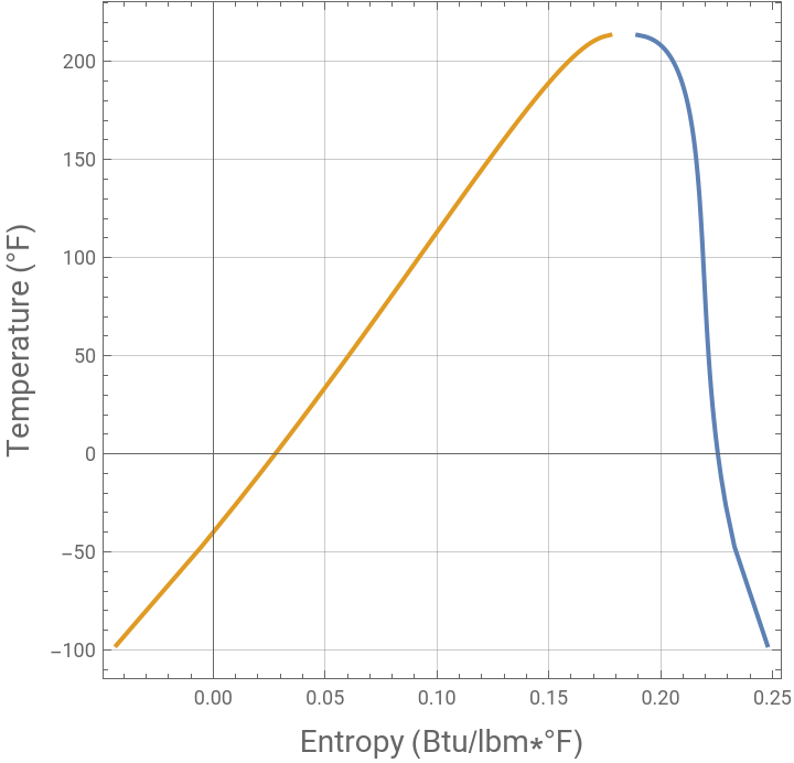
plt2=ListPlot[{tblsv1,tblsl1},JoinedTrue,FrameTrue,AspectRatio1,GridLinesAutomatic,FrameLabel{Style["Entropy (Btu/lbm*°F)",14],Style["Temperature (°F)",14]}]
Out[]=
In[]:=
Grid[{{"point","T °F","P psia","h Btu/lbm","s Btu/lbm*F","state"},{2,T2,P2,H2,S2,"sat. vap."},{3,T3,P3,H3,S3,"super heated vap."},{4,T4,P4,H4,S4,"sat. liq."},{1,T1,P1,H1,S1,quality}},Background{None,{Lighter[Yellow,.5],{White,Lighter[Blend[{Blue,Green}],.6]}}},Frame->All,ItemStyle12,Spacings{1.5,1.5}]
Out[]=
point | T °F | P psia | h Btu/lbm | s Btu/lbm*F | state |
2 | -55 | 17.3413 | 156.971 | 0.388195 | sat. vap. |
3 | 70.5826 | 63.9471 | 178.952 | 0.388195 | super heated vap. |
4 | 0 | 63.9471 | 15.6688 | 0.0354283 | sat. liq. |
1 | -55 | 17.3413 | 15.6688 | 0.0390305 | 0.1316 |
In[]:=
tblpt=Table[{datasat[[i]][[2]],datasat[[i]][[1]]},{i,1,Length[datasat]}];
In[]:=
fpt=Interpolation[tblpt];
In[]:=
FindRoot[fpt[x]==-10,{x,10}]
Out[]=
{x16.6276}
In[]:=
FindRoot[fpt[x]==90,{x,10}]
Out[]=
{x119.014}
In[]:=
H4=fhl[119.014]
Out[]=
41.6455
In[]:=
S4=fsl[119.014]
Out[]=
0.0856462
In[]:=
H2=fhv[16.6276]
Out[]=
101.682
In[]:=
S2=fsv[16.6276]
Out[]=
0.226775
In[]:=
H1=H4
Out[]=
41.6455
hlsat@P1<H1<hvsat@P1 --- Point 1 is in the two-phase region
In[]:=
H1
Out[]=
41.6455
Let us determine the COP of the refrigeration cycle if compressor is only 75% efficient
The OVC Cycle drawn on the H-P diagram
The OVC Cycle drawn on the T-S diagram
CYCLE 1
CYCLE 1
saturation properties - pressure increment = 5 psia
Temperature (F), Pressure (psia), Enthalpy (Btu/lbm), Entropy (Btu/lbm*R), Enthalpy (Btu/lbm), Entropy (Btu/lbm*R)
Temperature (F), Pressure (psia), Enthalpy (Btu/lbm), Entropy (Btu/lbm*R), Enthalpy (Btu/lbm), Entropy (Btu/lbm*R)
isobaric properties - pressure = 63.9473 psia
{Temperature (F), Pressure (psia), Enthalpy (Btu/lbm), Entropy (Btu/lbm*R), State)}
{Temperature (F), Pressure (psia), Enthalpy (Btu/lbm), Entropy (Btu/lbm*R), State)}
hlsat@P1<H1<hvsat@P1 --- Point 1 is in the two-phase region
Let us determine the COP of the refrigeration cycle if compressor is only 75% efficient
The OVC Cycle drawn on the H-P diagram
The OVC Cycle drawn on the T-S diagram
For a cooling rate of 200 BTU/s at–55 °F, let us determine (1) the flow rates of tetrafluoroethane and difluoromethane (in lb/s), (2) the power requirements for operation of each of the compressors, (3) the heat output from the condenser in Cycle 1 (in BTU/s) and (5) the overall COP
References
References
◼
[1] J.M. Smith, Hendrick Van Ness, Michael Abbott and Mark Swihart, Introduction to Chemical Engineering Thermodynamics, 9th Edition, NY: McGraw Hill, 2022.
CITE THIS NOTEBOOK
CITE THIS NOTEBOOK
Two-stage cascade refrigeration system
by Housam Binous and Ahmed Bellagi
Wolfram Community, STAFF PICKS, January 27, 2025
https://community.wolfram.com/groups/-/m/t/3364571
by Housam Binous and Ahmed Bellagi
Wolfram Community, STAFF PICKS, January 27, 2025
https://community.wolfram.com/groups/-/m/t/3364571