Abstract:
The specific transformation rules chosen for a given Wolfram Physics Model effects the types of structures it generates. Given the wide variety of physics phenomena that is being explored with Wolfram Models, it is important to determine the best model to study for any given physics property. A wolfram model that exhibits slow-growth is one example of an interesting model, because it mirrors the growth of our Universe. To find such models, a metric for growth is be defined, an appropriate graph layout will is developed, and many different transformation rule possibilities are be considered. In this project, I have found the tools to find Wolfram Models which exhibit slow-growth, and identified some interesting slow-growth rules.
The specific transformation rules chosen for a given Wolfram Physics Model effects the types of structures it generates. Given the wide variety of physics phenomena that is being explored with Wolfram Models, it is important to determine the best model to study for any given physics property. A wolfram model that exhibits slow-growth is one example of an interesting model, because it mirrors the growth of our Universe. To find such models, a metric for growth is be defined, an appropriate graph layout will is developed, and many different transformation rule possibilities are be considered. In this project, I have found the tools to find Wolfram Models which exhibit slow-growth, and identified some interesting slow-growth rules.
Thinking about Growth
Thinking about Growth
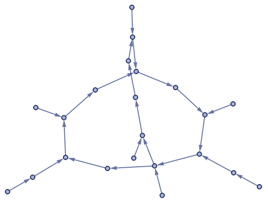
The image above shows all the possible connected Wolfram models with the rule signature: . There is one rule in this list that in unique among all the others, can you spot it? For n steps, this rule will grow at the rate of n^a Log(n). This unique rule, its hypergraph, and its growth rate are shown below:
2
2
3
2
{{1,2},{3,2}}{{4,1},{1,3},{3,2}}
|
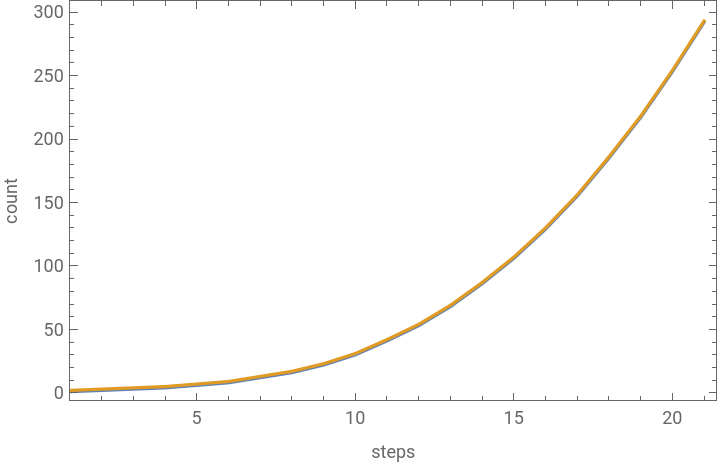
After evolving this hyper graph for many more steps, the following “lady bug” hypergraph emerges:
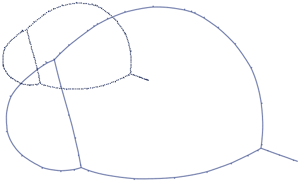

It came as a surprising result that this simple lady bug does not grow at linear or exponential rate like all the other hypergraphs. This interesting rule could not have been found without the help of the FindGrowth function
2
2
3
2
FindGrowth[Data_,option_:1,prop_:0] := Module[{ModelFits,ChosenModel,O},ModelFits = Range[7];ModelFits[[1]]= NonlinearModelFit[Data,aa x+bb,{aa,bb},x];ModelFits[[2]]= NonlinearModelFit[Data,aa*Exp[bb*x]+cc,{aa,bb,cc},x];ModelFits[[3]]= NonlinearModelFit[Data,aa*Log[x]+bb,{aa,bb},x];ModelFits[[4]]= NonlinearModelFit[Data,aa*x^2 + bb*x + cc,{aa,bb,cc},x];ModelFits[[5]]= NonlinearModelFit[Data, aa * x* Log[x] + bb,{aa,bb},x];ModelFits[[6]]= NonlinearModelFit[Data,aa * x^bb* Log[x]+cc,{aa,bb,cc},x];ModelFits[[7]]= NonlinearModelFit[Data, aa/(1+Exp[bb x])+cc,{aa,bb,cc},x];If[option == 1,O={Which[ModelFits[[1]]["RSquared"]> 0.999, ChosenModel = ModelFits[[1]]; "Linear",ModelFits[[2]]["RSquared"]> 0.999, ChosenModel = ModelFits[[2]];"Exponential",ModelFits[[3]]["RSquared"]> 0.999, ChosenModel = ModelFits[[3]];"Logarithmic",ModelFits[[4]]["RSquared"]> 0.999, ChosenModel = ModelFits[[4]];"Quadratic",ModelFits[[5]]["RSquared"]> 0.999, ChosenModel = ModelFits[[5]];"n*log(n)",ModelFits[[6]]["RSquared"]> 0.999, ChosenModel = ModelFits[[6]];"n^a*log(n)",ModelFits[[7]]["RSquared"]> 0.999, ChosenModel = ModelFits[[7]];"Logistic",True,"Other"]}];If[option 2,Module[{Residuals},Residuals = Total[#["FitResiduals"]^2]&/@ModelFits;O = {Which[Min[Residuals] Residuals[[1]], ChosenModel = ModelFits[[1]]; "Linear",Min[Residuals] Residuals[[2]], ChosenModel = ModelFits[[2]];"Exponential",Min[Residuals] Residuals[[3]], ChosenModel = ModelFits[[3]];"Logarithmic",Min[Residuals] Residuals[[4]], ChosenModel = ModelFits[[4]];"Quadratic",Min[Residuals] Residuals[[5]], ChosenModel = ModelFits[[5]];"n*log(n)",Min[Residuals] Residuals[[6]], ChosenModel = ModelFits[[6]];"n^a*log(n)",Min[Residuals] Residuals[[7]], ChosenModel = ModelFits[[7]];"Logistic",True, "Other"]}]];If[prop "PlotFits",AppendTo[O,Show[ListPlot[Style[Data,Red,Bold]],Flatten[Plot[#[x],{x,0,Length[Data]}]&/@ModelFits],Plot[Style[ChosenModel[x],Red,Bold],{x,0,Length[Data]}]]]];If[prop "ChosenModel",AppendTo[O,ChosenModel]];O]
FindGrowth is given a list of data points and automatically determines their growth rate. It will return “Linear”, “Exponential”, “Logarithmic”, “Quadratic”, “n*log(n)”, “n^a*log(n), “ Logistic “, or “ Other “ depending on which type of fitted curve best fits the data. The beauty about this function is that it can be combined with the outputs of the Wolfram Model Object to quickly identify interesting growth rates.
Considering Multiple Rules
Considering Multiple Rules
Multiple Rule Wolfram Models are the obvious place to look for interesting growth rates. The major challenge is that the complexity of possible rules balloons significantly when multiple rules are considered. The analysis of this project only considers only 1, 2, and 3 binary relation rules, and more than 22 quadrillion possibilities exist!
In[]:=
RuleG1=ResourceFunction["EnumerateWolframModelRules"][{{1,2}}{{2,2}}];RuleG2=ResourceFunction["EnumerateWolframModelRules"][{{1,2}}{{3,2}}];RuleG3=ResourceFunction["EnumerateWolframModelRules"][{{2,2}}{{3,2}}];RuleD1=ResourceFunction["EnumerateWolframModelRules"][{{2,2}}{{1,2}}];RuleD2=ResourceFunction["EnumerateWolframModelRules"][{{3,2}}{{1,2}}];RuleD3=ResourceFunction["EnumerateWolframModelRules"][{{3,2}}{{2,2}}];
In[]:=
Module[{G1,G2,G3,D1,D2,D3},G1=Length[RuleG1];G2=Length[RuleG2];G3=Length[RuleG3];D1=Length[RuleD1];D2=Length[RuleD2];D3=Length[RuleD3];((G3+1)*(G2+1)*(G1+1)-1)*((D1+1)*(D2+1)*(D3+1)-1)]
Out[]=
22425611608355632
There are many possible strategies to help navigate all these rules. In this project, I will be using the FindGrowth Function in addition to random sampling. Ideas for additional searching strategies are included in the Future Work section.
Results:
Results:
Signature : {{{1, 2}} {{2, 2}}, {{2, 2}} {{1, 2}}}
Signature : {{{1, 2}} {{2, 2}}, {{2, 2}} {{1, 2}}}
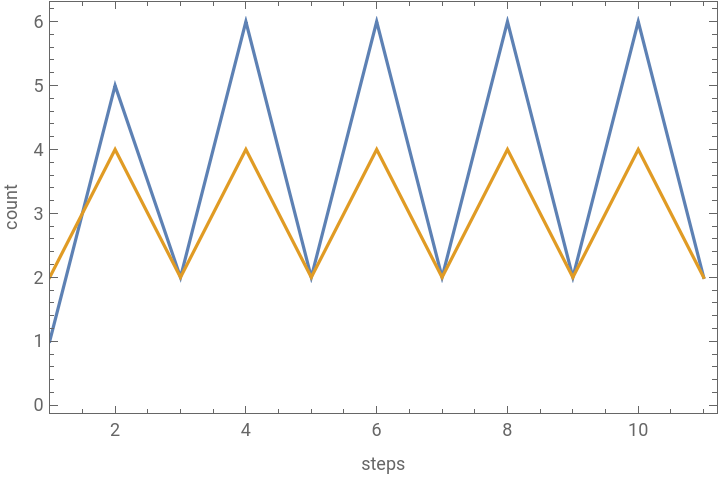
No interesting cases rules are found. All unique growth rules either terminate early or oscillate forever. Some examples:
{{{1,1}}{{2,1},{1,3}},{{1,2},{2,3}}{{3,3}}},
{{{1,1}}{{1,2},{2,3}},{{1,2},{2,3}}{{2,2}}},
,



,

Signature : {{{1, 2}} {{3, 2}}, {{2, 2}} {{1, 2}}}
Signature : {{{1, 2}} {{3, 2}}, {{2, 2}} {{1, 2}}}
Some interesting growth rates start to emerge. Still, the observed rules only all have final plots consisting of many simple disconnected graphs.
Signature : {{{2, 2}} {{3, 2}}, {{2, 2}} {{1, 2}}}
Signature : {{{2, 2}} {{3, 2}}, {{2, 2}} {{1, 2}}}
Now very interesting behavior begins to occur. Final States with structure, some odd growth rates, and an example of quadratic growth.
The rule below terminates early, but still the growth looks interesting:
First case of Quadratic Growth:
Due to a constraint in computational resources, only 1000 random rules were tested. I am certain additional interesting behavior can be found with additional sampling {{{2,2}}{{3,2}},{{2,2}}{{1,2}}} rules.
Signature : {{{2, 2}} {{3, 2}}, {{3, 2}} {{1, 2}}}
Signature : {{{2, 2}} {{3, 2}}, {{3, 2}} {{1, 2}}}
Many, cases of non-linear and non-exponential growth rates emerge. Many have been filtered out because they terminate or repeat. The rules that remain show the most interesting behavior.
“Other“ Growth:
Quadratic Growth:
Quadratic Growth:
Quadratic Growth:
Again, the amount of rules considered was constrained by computational resources. More interesting growth behavior can likely be found with additional random sampling of {{{2, 2}} -> {{3, 2}}, {{3, 2}} -> {{1, 2}}} rules.
Conclusion:
Conclusion:
Although linear or exponential growth is most common, there are many additional growth rates that are possible for Wolfram Models. Many binary relation rules have been identified which exhibit slow or unique growth rates. Perhaps more importantly, tools have been developed to automatically identify rules that exbibit potentially interesting growth rates.
Future Work:
Future Work:
Further analysis of the rules identified in this project may lead to some interesting physics results. Slow-growth universes are ideal for the exploration of concepts such as casual invariance, entropy, and universe growth rates.
There still remains many cases of interesting growth rates which have not yet been identified. Most simply, further random sampling of these rule sets may uncover some results. For more complicated rules, additional strategies may be considered to further optimize the search for slow-growth rules. These strategies include: reducing the number of starting rules, cannibalization of msultiple rule systems, and stricter model filtering.
There still remains many cases of interesting growth rates which have not yet been identified. Most simply, further random sampling of these rule sets may uncover some results. For more complicated rules, additional strategies may be considered to further optimize the search for slow-growth rules. These strategies include: reducing the number of starting rules, cannibalization of msultiple rule systems, and stricter model filtering.
Acknowledgment
Acknowledgment
Mentor: I would like to thank Jack Hermrath for his guidance on this project
I would also like to thank Jin Yan and Jatin Kansal for their discussions and collaborations.
References
References
◼
WOLFRAM, S., 2020. PROJECT TO FIND THE FUNDAMENTAL THEORY OF PHYSICS. [S.l.]: WOLFRAM MEDIA INC.