In[]:=
OrthopticCurveEllipse::usage="It is the geometric locus of the intersection point of two tangent lines to a curve and orthogonal to each other. References: Personal.";
Development:
Obtaining the cartesian equation from the orthoptic curve to the parabola (observe that quadratic terms form a perfect square trinomiam, there is no doubt that it is a conical of the parabola gender):
In[]:=
4-4xy+-4x-8y-4==0;y-==m(x-);y==+mx-m;4-4x(+mx-m)+-4x-8(+mx-m)-4==0;Expand[4-4x(+mx-m)+-4x-8(+mx-m)-4==0]
2
x
2
y
y
0
x
0
y
0
x
0
2
x
y
0
x
0
2
(+mx-m)
y
0
x
0
y
0
x
0
2
x
y
0
x
0
2
(+mx-m)
y
0
x
0
y
0
x
0
Out[]=
-4-4x-8mx+4-4m++8m+4mx-2x+-8-4x+2mx-2m+0
2
x
2
x
2
m
2
x
x
0
x
0
2
m
x
0
2
m
2
x
0
y
0
y
0
y
0
x
0
y
0
2
y
0
In[]:=
-4-4x-8mx+4-4m++8m+4mx-2x+-8-4x+2mx-2m+0;(4-4m+)+-4-8m+4m-2-4+2mx-4+8m+-8-2m+==0;
2
x
2
x
2
m
2
x
x
0
x
0
2
m
x
0
2
m
2
x
0
y
0
y
0
y
0
x
0
y
0
2
y
0
2
m
2
x
x
0
2
m
x
0
y
0
y
0
x
0
2
m
2
x
0
y
0
x
0
y
0
2
y
0
Due to the condition of tangency, the discriminant must be zero:
In[]:=
SimplifyExpand-4(4-4m+)-4+8m+-8-2m+==0
2
-4-8m+4m-2-4+2m
x
0
2
m
x
0
y
0
y
0
2
m
x
0
2
m
2
x
0
y
0
x
0
y
0
2
y
0
Out[]=
1++(-2+m)m(-2+m)
2
m
x
0
y
0
In[]:=
1++(-2+m)m(-2+m);(1+)+(-2-)m+2+1==0;
2
m
x
0
y
0
x
0
2
m
x
0
y
0
y
0
By Vieta’s theorem:
In[]:=
m
1
m
2
c
a
Due to the perpendicularity condition:
In[]:=
2+1
y
0
1+
x
0
x
0
y
0
The orthoptic “curve” as expected, corresponds to the directrix of the parabola.
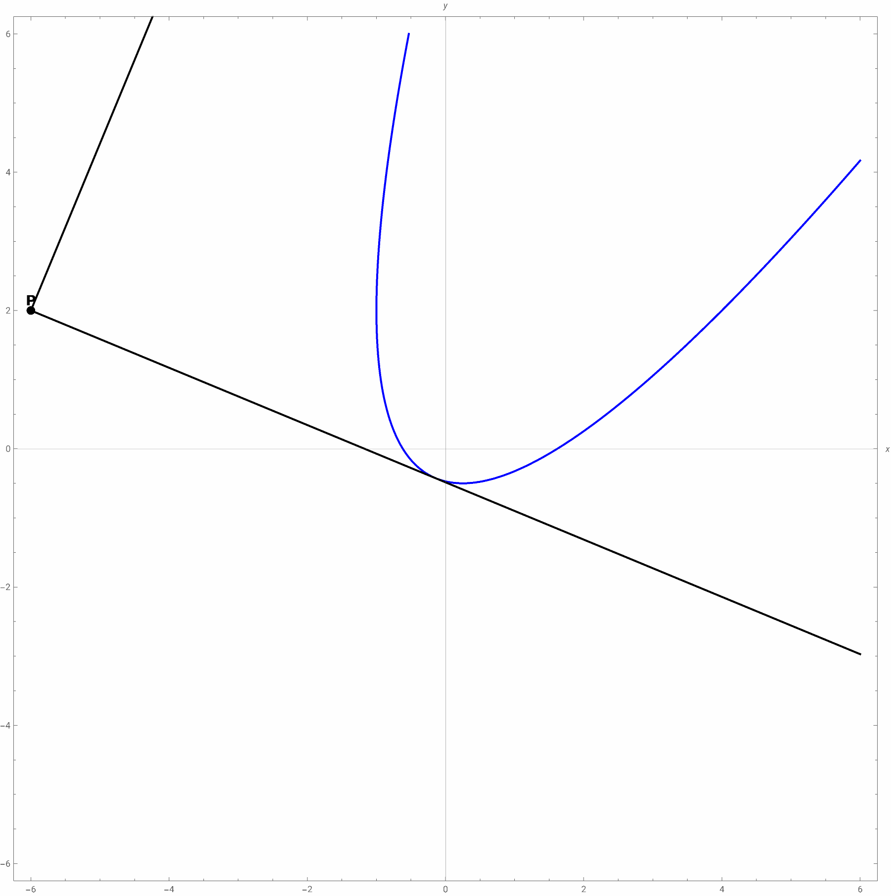
Animation:
In[]:=
ManipulateModule{p,slopes,m1,m2,t1Line,t2Line},p=t1,-+1;slopes=m/.Solve[(1+p[[1]])+(-2p[[1]]-p[[2]])m+2p[[2]]+1==0,m]//Simplify;{m1,m2}=slopes;t1Line[x_]:=p[[2]]+m1(x-p[[1]]);t2Line[x_]:=p[[2]]+m2(x-p[[1]]);ShowContourPlot[4-4xy+-4x-8y-4==0,{x,-6,6},{y,-6,6},PerformanceGoal->"Quality",PlotPoints60,ContourStyle->{Blue,Thick}],ParametricPlotx,-+1,{x,-6,t1},ColorFunction->Function[{x,y,u},ColorData["BlueGreenYellow"][u]],ColorFunctionScaling->True,Plot[t1Line[x],{x,-6,6},PlotStyle->Black],Plot[t2Line[x],{x,-6,6},PlotStyle->Black],Graphics[{Black,PointSize[0.01],Point[p],Text[Style["P",14,Bold],p,{0,-1.2}]}],AspectRatio->Automatic,Axes->True,AxesOrigin->{0,0},AxesLabel->{x,y},PlotRange->6,ImageSize->900,{{t1,-6+0.00002,"Value t1"},-6+0.000001,6,0.00001},SaveDefinitions->True
t1
2
2
m
2
x
2
y
x
2
Out[]=