Sinc Interpolation for Signal Reconstruction

sampling frequency (Hz)

signal to sample

sawtooth wave

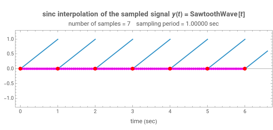
This Demonstration illustrates the use of the sinc interpolation formula to reconstruct a continuous signal from some of its samples. The formula provides exact reconstructions for signals that are bandlimited and whose samples were obtained using the required Nyquist sampling frequency, to eliminate aliasing in the reconstruction of the signal.

You can apply the interpolation formula to a number of continuous signals. Increasing the sampling frequency gives a more accurate reconstruction of the continuous function.

The original signal is shown as a blue solid line and the sample locations are shown by red circles. The reconstructed signal is shown using the dotted magenta line and is superimposed on the original signal to make it easier to see the effect of increasing the sampling frequency on the reconstruction of the original signal from its samples.

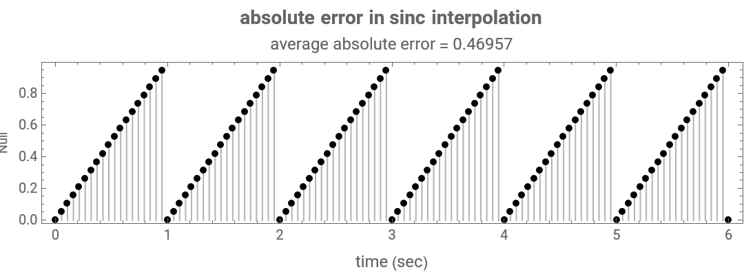
Because the number of samples is limited, there will be some error in the reconstruction, even at a higher sampling frequency than the Nyquist frequency. The absolute (point by point) error shown by the original signal and the reconstructed signal is plotted to show how the error decreases as the sampling rate increases.

Details

The function

sinc(x)

is defined by

sinc(x)=sin(x)/x

for

x≠0

, with

sinc(0)=1

. The sinc interpolation formula is defined as

x(t)=

∞

∑

n=-∞

sinc

(t-nT)

, where

is the sampling period used to determine

from the original signal, and

x(t)

is the reconstructed signal. The above formula represents a linear convolution between the sequence

and scaled and shifted samples of the

sinc

function. In this Demonstration, a limited number of samples

are generated, and the above sum is carried out for

samples, labeled from

k=0

k=N-1

. Due to the shifting of the

sinc

function by integer multiples of

, this results in

x(t)

having the exact value of a sample located at a multiple of

. This can be seen by observing that the absolute error is always zero at times which are integer multiples of

, in other words at the sample locations. In this implementation, the

sinc

function is sampled at a much higher rate than the sampling frequency used for the original function, in order to produce a smoother plotted result.

A. V. Oppenheim and R. W. Schafer, Digital Signal Processing, Englewood Cliffs, NJ: Prentice Hall, 1975.

External Links

Sinc Function (Wolfram MathWorld)

Nyquist Frequency (Wolfram MathWorld)

Permanent Citation

Nasser M. Abbasi

"Sinc Interpolation for Signal Reconstruction"
http://demonstrations.wolfram.com/SincInterpolationForSignalReconstruction/
Wolfram Demonstrations Project
Published: March 7, 2011