An analytical solution for the potential field due to a uniformly charged rectangular plate has been examined in the following two recent articles :
1. D . A . Fagundes, "Electrostatic potential of a rectangular uniformly charged plate: exact solution and limiting cases," Euro . J . Phys. 43, 015203 (2021).
2. O. Ciftja and B. Ciftja, “Exact analytical results for the electrostatic potential due to a uniformly charged finite plate,” Can. J. Phys. 101, 607-6012 (2023).
In Ref. [2] , the potential V(x,y,z) for a finite rectangular plate lying on the x-y plane has been brought to the one-dimensional integral expression in Eq. (10). Only limiting results for V(0,0,z) are derived explicitly. Using a different approach, the same limiting potential V(0,0,z) has been obtained in Ref [1].
It is the goal in this note to show that using Mathematica one can obtain the potential field and the corresponding electric field at an arbitrary point in space.
The potential field due to a uniformly charged rectangular plate of dimensions 2a and 2b is given as follows:
It is the goal in this note to show that using Mathematica one can obtain the potential field and the corresponding electric field at an arbitrary point in space.
The potential field due to a uniformly charged rectangular plate of dimensions 2a and 2b is given as follows:
V(x,y,z)=y'x'++;
σ
4πϵ
b
∫
-b
a
∫
-a
1
2
(x-x')
2
(y-y')
2
z
σ is the constant charge surface on the plate and ϵ denotes the permittivity .
The change of variables
x - x' = X, y - y' = Y
results in the expression
V(x,y,z)=YX++.
σ
4πϵ
y+b
∫
y-b
x+a
∫
x-a
1
2
X
2
Y
2
z
The integration over X is performed first .
V(x,y,z)=YX++
σ
4πϵ
x+a
∫
x-a
1
2
X
2
Y
2
z
Integrate++,{X,x-a,x+a}
1
2
X
2
Y
2
z
This expression is rewritten a follows :
Log;
a+x+++
2
Y
2
(a+x)
2
z
-a+x+++
2
Y
2
(a-x)
2
z
The integration over Y is performed next .
IntegrateLog,{Y,y-b,y+b}
a+x+++
2
Y
2
(a+x)
2
z
-a+x+++
2
Y
2
(a-x)
2
z
This solution is simplified as follows:
V=-zArcTan+ArcTan+ArcTan+ArcTan+(b-y)Log+(a-x)Log-(b+y)Log+(a+x)Log;
σ
4πϵ
(a-x)(b-y)
z++
2
(a-x)
2
(b-y)
2
z
(a+x)(b-y)
z++
2
(a+x)
2
(b-y)
2
z
(a-x)(b+y)
z++
2
(a-x)
2
(b+y)
2
z
(a+x)(b+y)
z++
2
(a+x)
2
(b+y)
2
z
a+x+++
2
(a+x)
2
(b-y)
2
z
-a+x+++
2
(a-x)
2
(b-y)
2
z
b+y+++
2
(a-x)
2
(b+y)
2
z
-b+y+++
2
(a-x)
2
(b-y)
2
z
-a+x+++
2
(a-x)
2
(b+y)
2
z
a+x+++
2
(a+x)
2
(b+y)
2
z
b+y+++
2
(a+x)
2
(b+y)
2
z
-b+y+++
2
(a+x)
2
(b-y)
2
z
This is the potential field V (x, y, z) at an arbitrary point in space .
Along the axis of symmetry one has
V/.x->0/.y->0//FullSimplify
1
4πϵ
ab
z++
2
a
2
b
2
z
-a+++
2
a
2
b
2
z
a+++
2
a
2
b
2
z
a+++
2
a
2
b
2
z
-a+++
2
a
2
b
2
z
b+++
2
a
2
b
2
z
-b+++
2
a
2
b
2
z
or, more simply,
V0=σ-4zArcTan+bLog+2aLog;
1
4πϵ
ab
z++
2
a
2
b
2
z
2
a+++
2
a
2
b
2
z
2
-a+++
2
a
2
b
2
z
b+++
2
a
2
b
2
z
-b+++
2
a
2
b
2
z
This expression coincides with those given in the Refs [1] and [2].
R12=4aArcSinh+bArcSinh-zArcTan;
σ
4πϵ
b
z^2+a^2
a
z^2+b^2
ab
z
z^2+a^2+b^2
V0/.{a->1,b->2,z->2}//N
0.271953σ
ϵ
R12/.{a->1,b->2,z->2}//N
0.271953σ
ϵ
The exact electric field at an arbitrary point is given by
e=-Grad[V,{x,y,z}];
e1=e/.y->0/.a->1/.b->2;
σ
4πϵ
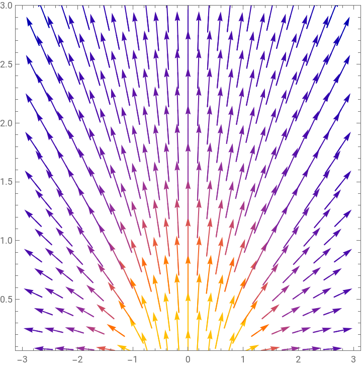
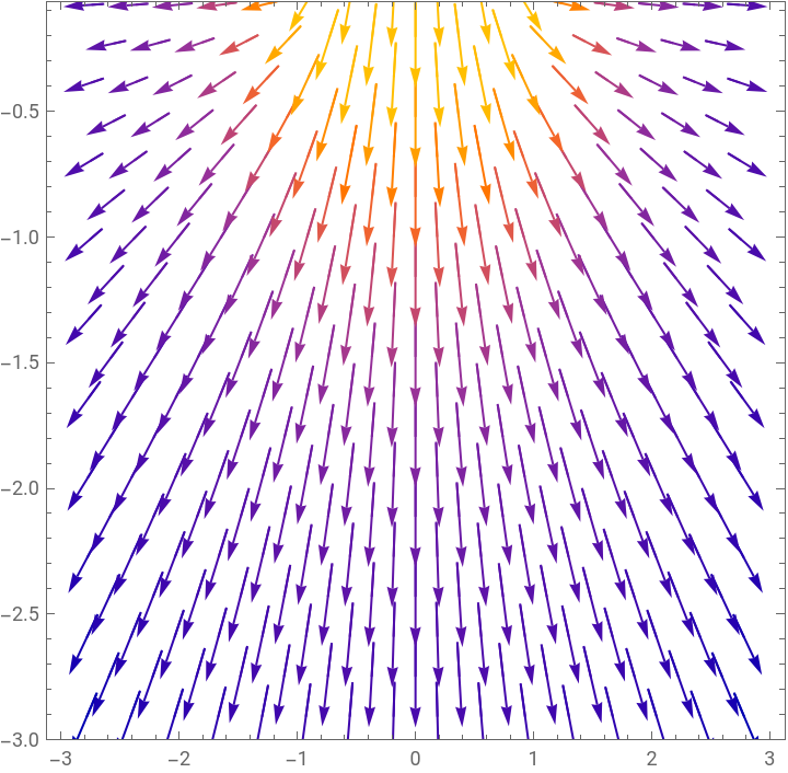
Below,vectorplotsoftheelectricfeldareshownonthey=0plane.
e1=e/.y->0/.a->1/.b->2;
σ
4πϵ
VectorPlot[{e1.{1,0,0},e1.{0,0,1}},{x,-3,3},{z,-3,3},PlotRange->{1/16,3}]
VectorPlot[{e1.{1,0,0},e1.{0,0,1}},{x,-3,3},{z,-3,3},PlotRange->{-3,-1/16}]
The electric field along the axis of symmetry is given as follows :
e0=-Grad[Sol,{x,y,z}]/.{x->0,y->0}//FullSimplify
σ
4πϵ
0,,
σLog+Log
-a+++
2
a
2
b
2
z
a+++
2
a
2
b
2
z
a+++
2
a
2
b
2
z
-a+++
2
a
2
b
2
z
4πϵ
σArcTan
ab
z++
2
a
2
b
2
z
πϵ
The z - component is identical to that given in Eq. (5) of Ref. [1] obtained from -dV(0,0,z)/dz.
CITE THIS NOTEBOOK
CITE THIS NOTEBOOK
Potential field of a charged rectangular plate
by Ioannis M. Besieris
Wolfram Community, STAFF PICKS, November 4, 2025
https://community.wolfram.com/groups/-/m/t/3570273
by Ioannis M. Besieris
Wolfram Community, STAFF PICKS, November 4, 2025
https://community.wolfram.com/groups/-/m/t/3570273