Analog quantum processing units (quantum annealers) use continuous variables for optimization tasks, such as finding global minima. Gate-based quantum computers use discrete quantum gates to manipulate qubits for versatile quantum algorithms, including factorization, simulation, and optimization. One example of analog Quantum Processing Units (QPUs) is Aquila, which is a neutral-atom QPU from QuEra Computing, with up to 256 qubit. Aquila is also available on Amazon Braket, which is accessible using AWS service connect from a Wolfram notebook. In this computational essay, we will focus on some examples from QuEra's recent white paper, and do the simulation using quantum functionalities of Wolfram quantum framework, and also show how to send queries to Aquila, using Amazon Braket.
This notebook has been published in the Wolfram Community, too: https://community.wolfram.com/groups/-/m/t/2983137

where is the the Rabi frequency, the laser phase, and the detuning of the driving laser field coupling the ground states and excited Rydberg state of the j-th atom. - represents the van der Waals interaction between atom-j and atom-k, while is the number operator of j-th site (more info on actual values of can be found in QuEra webpages).
Ω
ϕ
Δ
g
j
r
j
V
jk
C
6
x
j
x
k
6
|
n
j
r
j
r
j
C
6
We have defined the corresponding Hamiltonian as follows: , where it takes sites as a list of atom positions, , with each position in μm, is the the Rabi frequency, the laser phase, and the detuning of the driving laser field.
AquilaHamiltonian[sites, {Ω, Δ, ϕ}]
{{,},{,},...}
x
1
y
1
x
2
y
2
Ω
ϕ
Δ
Single atom
Single atom
Let’s consider the single atom dynamics.
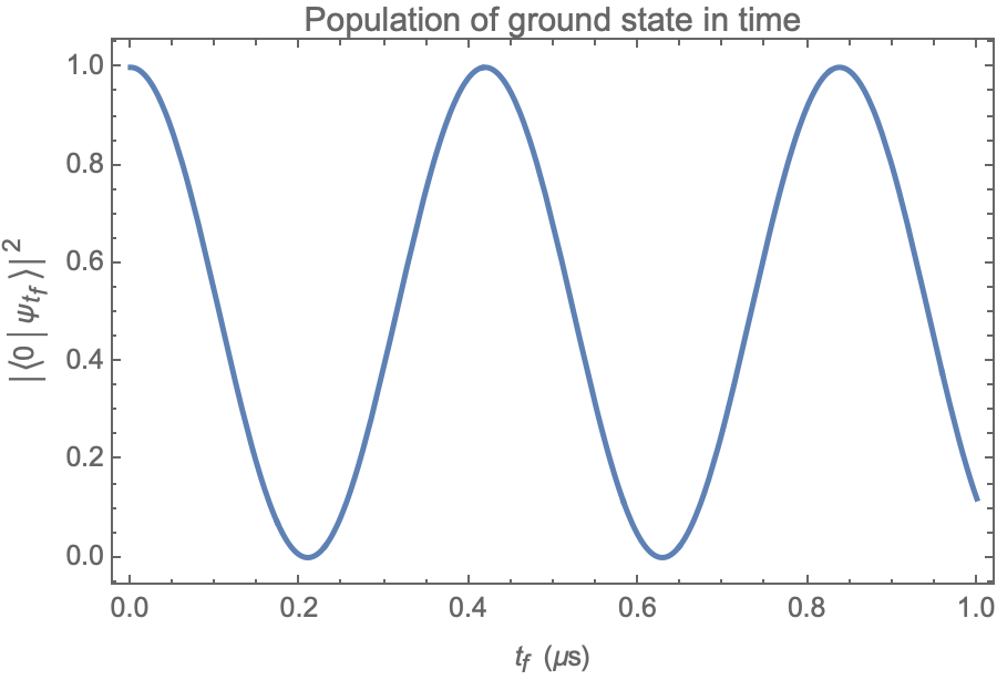
Rabi Oscillation (Ω=constant, Δ=0 and ϕ=0)
Rabi Oscillation (Ω=constant, Δ=0 and ϕ=0)
For this case, one can get the state symbolically.
In[]:=
ψ1RO=QuantumEvolve[AquilaHamiltonian[{{0,0}},{15.,0,0}],t]
Out[]=

As an example, calculate the populations at
t=1μs
In[]:=
ψ1RO[1.]["Probability"]
Out[]=
|0〉0.120156,|1〉0.879844
Population of ground state as a function of time:
In[]:=
Plotψ1RO["Probability"][[1]],{t,0,1},FrameLabel->" (μs)",,Frame->True,PlotLabel->"Population of ground state in time"
t
f
2
0
""
ψ
t
f
Out[]=
Ramsey Protocol (Ω as two pulses, Δ=constant, ϕ=0)
Ramsey Protocol (Ω as two pulses, Δ=constant, ϕ=0)
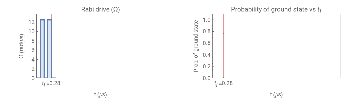
For this protocol, the atom is driven by two pulses, with a hold time between pulses, and Δ and ϕ are set to zero.
In[]:=
pulses[{amplitude_,δt_,gap_},t_]:=
;
|
In[]:=
In[]:=
data=Module{δt=.1,amplitude=12.5,plotRabi,plotProb,state,prob={}},Tablestate=QuantumEvolve[AquilaHamiltonian[{{0,0}},{pulses[{amplitude,δt,gap},t],10.5,0}],{t,0,4}];plotRabi=Plotpulses[{amplitude,δt,gap},t],{t,-δt,2δt+gap},;prob=Join[prob,{{δt+gap,state[δt+gap]["Probability"][[1]]}}];plotProb=ListLinePlotprob,;{plotRabi,plotProb},{gap,Range[.18,3,.1]};
In[]:=
ListAnimate[images=GraphicsRow[#,ImageSize->Large]&/@data]
Out[]=
Floquet Protocol (Ω=const., Δ=const. Sin[ω t], and ϕ=0)
Floquet Protocol (Ω=const., Δ=const. Sin[ω t], and ϕ=0)
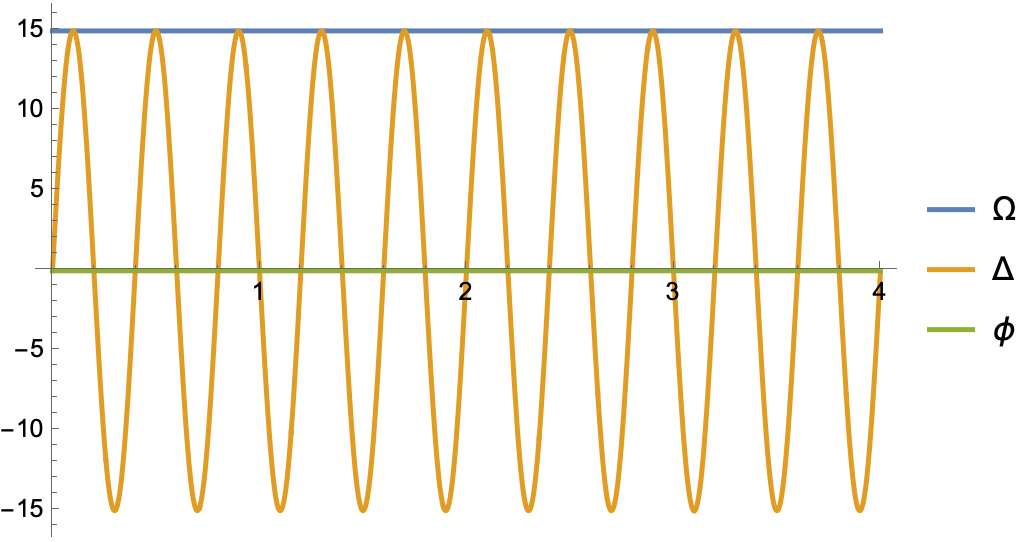
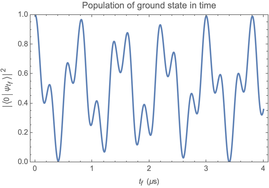
In this scenario, the Rabi drive remains constant, and the detuning oscillates sinusoidally over time, with a phase set to zero.
In[]:=
Plot[{15.,15.Sin[5πt],0},{t,0,4},PlotLegends->{"Ω","Δ","ϕ"}]
Out[]=
In[]:=
ψFlo=QuantumEvolve[AquilaHamiltonian[{{0,0}},{15.,15.Sin[5πt],0}],{t,0,4}];
Population per site (keys are site labels (qubits) and values are population):
In[]:=
PlotψFlo[t]["Probability"][[1]],{t,0,4},PlotRange->{0,1},FrameLabel->" (μs)",,Frame->True,PlotLabel->"Population of ground state in time"
t
f
2
0
""
ψ
t
f
Out[]=
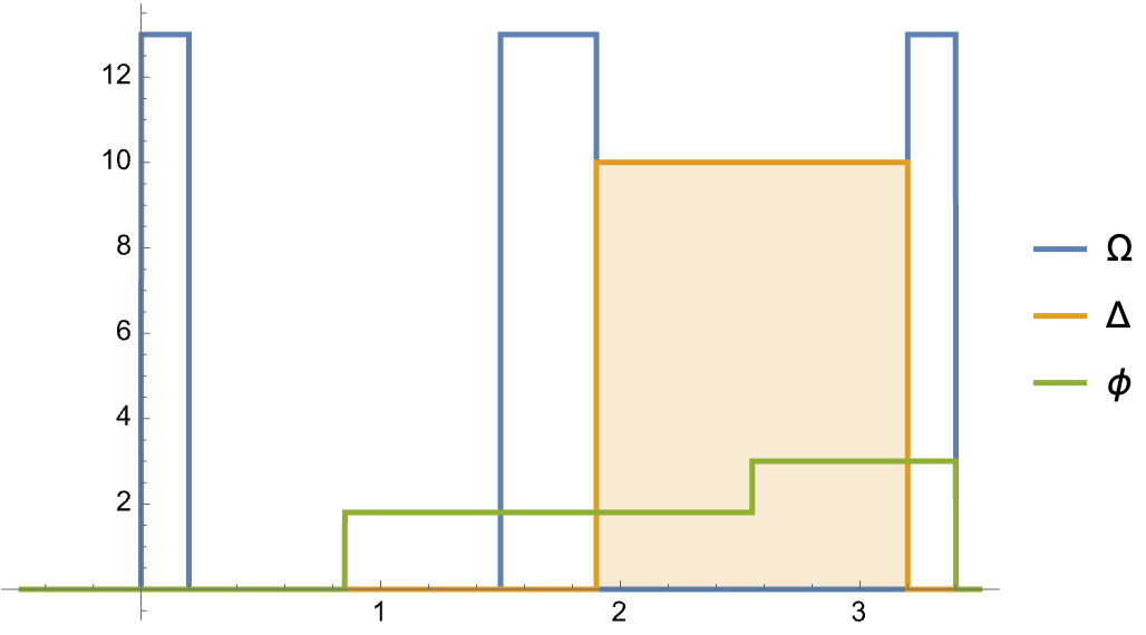
Spin echo
Spin echo
In[]:=
ClearAll[Ω,Δ,ϕ];Ω[{δt_,gap_},t_]:=
;Δ[{δt_,gap_},t_]:=
;ϕ[{δt_,gap_},t_]:=
;
13. | 0<=t<=δt||δt+gap<=t<=3δt+gap||3δt+2gap<=t<=4δt+2gap |
0 | True |
10 | 3δt+gap<=t<=3δt+2gap |
0 | True |
|
In[]:=
δt=.2;With[{gap=1.3},Plot[{Ω[{δt,gap},t],Δ[{δt,gap},t],ϕ[{δt,gap},t]},{t,-.5,3.5},Exclusions->None,PlotRange->All,PlotPoints100,PlotLegends->{"Ω","Δ","ϕ"},Filling{2Axis}]]
Out[]=
Two atoms
Two atoms
Rydberg blockade radius
Rydberg blockade radius
Levine-Pichler gate analogues
Levine-Pichler gate analogues
Interacting non-equilibrium dynamics of two atoms
Interacting non-equilibrium dynamics of two atoms
Multi-atoms: ordered phases
Multi-atoms: ordered phases
Multi atoms: Blockaded Rabi Oscillations
Multi atoms: Blockaded Rabi Oscillations
The Rydberg blockade effect arises from the strong interactions between Rydberg atoms. When two or more Rydberg atoms are in close proximity, the strong interactions between them can prevent multiple atoms from simultaneously being excited to a Rydberg state. In other words, the excitation of one Rydberg atom can “block” the excitation of nearby atoms.
Define positions of atoms in a 2D lattice
Plot atoms’s lattice
Find the final quantum state vector, and wrap it around by a QuantumState:
Multi atoms: quantum scars
Multi atoms: quantum scars
Calculate the probability of Néel state 1010101010101 in time:
Plot it over time:
Maximum independent set on unit disk graphs
Maximum independent set on unit disk graphs
Let’s first analyze the Maximum independent set on unit disk graphs, classically.
Create a King’s graph with a 30% random dropout:
Show the King’s graph:
Find an independent vertex set of the King’s graph with a maximum number of vertices:
Highlight them in the graph:
Now, using a quantum algorithm, we will try to find those max independent vertices (in our case, it will be qubits 1, 3, 7 and 8, in a quantum system with 11 qubits).
Create the corresponding 2D lattice, with the distance of 5μm
Create the corresponding parameters of the Hamiltonian and plot them:
Find the time-dependent quantum state:
Bar-chart of probabilities of all independent vertex set,
Visualize it
Final Rydberg population per site at a given time:
Plot Rydberg population per sites over time:
AWS
AWS
In this section, we will send a query to QuEra Aquila, using Amazon Braket.
Site population:
Bit-string population
Send the job to QuEra Aquila:
Given preSequence with all 1 (meaning the initial preparation was done correctly)
[make sure I understand what does that mean, given the preSequence are not all 1111...]
[make sure I understand what does that mean, given the preSequence are not all 1111...]
Different of population between theory and experimental values for each site
CITE THIS NOTEBOOK
CITE THIS NOTEBOOK
Wolfram quantum framework for analog QPUs: QuEra Aquila case
by Mads Bahrami
Wolfram Community, STAFF PICKS, August 4, 2023
https://community.wolfram.com/groups/-/m/t/2983137
by Mads Bahrami
Wolfram Community, STAFF PICKS, August 4, 2023
https://community.wolfram.com/groups/-/m/t/2983137