Conventional methods in quantum computing rely on circuit-based methods with quantum gates. However, Farhi et al. introduced a new algorithm based on the adiabatic theorem using the transition between the ground states of two Hamiltonians to solve quantum optimization and search problems. This baseline approach achieved an runtime on the Grover search problem, which was improved to by Roland and Cerf via locally enforcing the adiabatic time condition at each timestep. However, both of these algorithms are ineffective when the energy gap between the ground state and first excited state is small. To combat this, counterdiabatic evolution was created, introducing counterdiabatic driving (CD) terms into the system’s Hamiltonian to absorb any nonadiabatic energy level transitions. Using these methods, I compare their runtime and fidelity scaling on the n-qubit Grover search problem. Future work should compute exact adiabatic gauge potential instead of relying on nested commutator approximations and theoretically prove why the Grover problem space limits the gauge potential expressivity.
O(N)
O(
N
)Introduction
Introduction
Before discussing the algorithms implemented in this project, it is necessary to understand some of the baseline topics of quantum mechanics and computing. A quantum system is, in simple terms, a system of objects that are governed by the laws of quantum mechanics. Instead of all objects having deterministic and continuous future states over time, quantum systems operate on rules such that their future behavior cannot be predicted, and their properties exist in discrete packets. These systems can typically be represented by a wavefunction, which is a mathematical representation (usually a vector) of the probabilities of all possible states within a quantum system.
In quantum computing, systems are represented by a set of quantum bits, or qubits. These qubits can be in a superposition of 0 and 1, meaning they have a probability to measure either 0 or 1. When multiple qubits are introduced into a system, the number of states grows exponentially, thereby making the system larger. For example, with 1 qubit there are 2 states: 0 or 1. But with 2 qubits, there are 4 states: 00, 01, 10, and 11. Similarly, for n qubits, there will be possiblebasisstatesofthesystem,wherenisthenumberofqubits.Here, the wavefunction will just be a vector with elements, where the square of each element corresponds to the probability of measuring it. A wavefunction can also be referred to as a quantum state or a statevector.
n
2
n
2
Quantum systems can also be associated to Hamiltonians, which is a mathematical operator (a matrix in this case) that corresponds to the total energy of a system. It represents all physical interactions and energy contributions. When measuring the total energy of a system, the possible outcomes (also known as energy levels) equal the eigenvalues of the Hamiltonian, each of which is correlated with an eigenvector representing a stable energy level. Specifically, the lowest energy level is called the ground state. Hamiltonians are also used in the Schrödinger equation to calculate how a quantum state will evolve over time, detailing how its probabilities will change temporally.
For working with quantum computing, I will be using the Wolfram Quantum Framework, which has many of the required functionalities for simulated quantum computing already built in.
In[]:=
PacletInstall["https://www.wolfr.am/DevWQCF",ForceVersionInstall->True];<<Wolfram`QuantumFramework`
Baseline Adiabatic Evolution
Baseline Adiabatic Evolution
The first algorithm I will analyze is the quantum adiabatic algorithm. This was introduced by Farhi et. al in 2000 [1] and was applied to the boolean satisfiability problem. While normal quantum computing relies on applying gates to quantum states and measuring the result, this algorithm relies on something else called the adiabatic theorem. This theorem states that a “physical system remains in its instantaneous eigenstate if a given perturbation is acting on it slowly enough and if there is a gap between the eigenvalue and the rest of the Hamiltonian’s spectrum” as stated in Born and Fock’s work from 1928. In simpler terms, if the system evolves slowly enough, a Hamiltonian will remain in the same eigenstate it is currently when it is evolving.
The algorithm exploits this through a novel technique: by making a system’s time-dependent Hamiltonian a mix of two other Hamiltonians. The first Hamiltonian is a problem Hamiltonian with weights and terms to represent the energy state of the problem. There is also a base Hamiltonian whose design is intentionally very simple—its ground state is easy to construct and find. The paper mixes the base Hamiltonian ) and the problem Hamiltonian ) via a simple linear interpolation: , where t is the current timestep, and T is the total evolution time. With this, the base Hamiltonian is applied at time 0, and slowly evolves into the problem Hamiltonian at the end time 1, so that the problem is solved during the evolution.
(
H
B
(
H
P
H(t)=1-+
t
T
H
B
t
T
H
P
Base Adiabatic Evolution for Grover Search
Base Adiabatic Evolution for Grover Search
Define number of qubits to use for simulation, and states needed to generate Hamiltonians:
In[]:=
qubits=2;psi0=QuantumState["UniformSuperposition"[qubits]];m=QuantumState["Register"[qubits,2]];
Define base Hamiltonian and problem Hamiltonian via projectors. M is the marked state for the Grover search:
H
0
H
m
In[]:=
h0=QuantumOperator[StringRepeat["I",qubits]]-psi0["Operator"];hm=QuantumOperator[StringRepeat["I",qubits]]-m["Operator"];
Show the and matrices.
H
0
H
m
In[]:=
Normal@h0["Matrix"]//TraditionalFormNormal@hm["Matrix"]//TraditionalForm
Out[]//TraditionalForm=
3 4 | - 1 4 | - 1 4 | - 1 4 |
- 1 4 | 3 4 | - 1 4 | - 1 4 |
- 1 4 | - 1 4 | 3 4 | - 1 4 |
- 1 4 | - 1 4 | - 1 4 | 3 4 |
Out[]//TraditionalForm=
1 | 0 | 0 | 0 |
0 | 1 | 0 | 0 |
0 | 0 | 0 | 0 |
0 | 0 | 0 | 1 |
Construct the time-dependent Hamiltonian, which is a linear mixture between the base and problem Hamiltonian:
H
s
In[]:=
ClearAll[hs]hs=QuantumOperator[(1-s)h0+shm,"Parameter"->s];
Spectral Gap and Coupling Analysis
Spectral Gap and Coupling Analysis
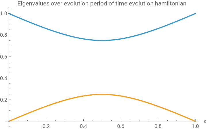
The time T is dependent on the gap between the lowest (ground state) and second lowest energy values of the time-dependent Hamiltonian. This is because if the system evolves too fast, according to the adiabatic theorem, it will jump into the first excited energy state of the Hamiltonian, and the system will no longer end up in the ground state of the final problem Hamiltonian. To account for this, the paper derives a minimum condition for T, which is , where is the minimum spectral gap between the ground state and the first energy level, and ξ is the expectation of the derivative of the time-dependent Hamiltonian with respect to (in other words, a measure of how strong the adiabatic coupling is). So, before running the algorithm, I will use this formula to calculate the minimum time T needed to maintain adiabicity for.
T>>
ξ
2
g
min
g
min
t
T
Compute the eigenvalues and extract the ground state and first excited state energy values:
In[]:=
curEigenvals=((1-s)*h0+s*hm)["Eigenvalues"];eigenval1=curEigenvals[[-1]]eigenval2=curEigenvals[[-2]]
Out[]=
1
2
1-3s+3
2
s
Out[]=
1
2
1-3s+3
2
s
The eigenvalue gap over the time period is plotted below, and the smallest gap is at around s = 0.5.
0≤s≤1
In[]:=
Plot{eigenval1,eigenval2},{s,0,1},
Out[]=


Minimize the difference between the eigenvalues to find the minimum gap:
In[]:=
symbolicGap=eigenval1-eigenval2;
In[]:=
minGap=Minimize[symbolicGap,s][[1]]
Out[]=
1
2
This minimum difference of 0.5 between the ground state and first energy level eigenvalues is seen in the paper, which says the gap equal to . N = dimension of space, or with n = number of qubits.
1
N
n
2
Now, the numerator of the condition on T, ξ needs the Hamiltonian’s eigenvectors for an expectation value: ℓ1;sℓ0;s. This represents how coupled the ground eigenstate and the first excited eigenstate are.
max
0≤s≤1
d
H
ds
Display associated eigenvalues and eigenvectors with the eigensystem command:
In[]:=
ClearAll[eigenvectors,eigensystem]eigensystem=hs[s]["Eigensystem"]
Out[]=
1,1,1-1+,0,0,-,,-,0,0,,,,,,,,
1
2
1-3s+3
,2
s
1
2
1-3s+3
,2
s
1
2
1
2
1
2
1
2
1
3+
2
Abs
1+
1-3s+3
2
s
1-2s+
1-3s+3
2
s
1
3+
2
Abs
1+
1-3s+3
2
s
1-2s+
1-3s+3
2
s
1+
1-3s+3
2
s
1-2s+
1-3s+3
2
s
3+
2
Abs
1+
1-3s+3
2
s
1-2s+
1-3s+3
2
s
1
3+
2
Abs
1+
1-3s+3
2
s
1-2s+
1-3s+3
2
s
1
3+
2
Abs
-1+
1-3s+3
2
s
-1+2s+
1-3s+3
2
s
1
3+
2
Abs
-1+
1-3s+3
2
s
-1+2s+
1-3s+3
2
s
-1+
1-3s+3
2
s
-1+2s+
1-3s+3
2
s
3+
2
Abs
-1+
1-3s+3
2
s
-1+2s+
1-3s+3
2
s
1
3+
2
Abs
-1+
1-3s+3
2
s
-1+2s+
1-3s+3
2
s
In[]:=
eigenvectors=hs[s]["Eigenvectors"];
An expectation value is squishing a quantum operator (which is just a matrix) between a row and a column vector. This can be computed through standard matrix multiplication.
Get the first excited eigenvector, and turn it into a row vector with the “Dagger” operation, also known as the complex conjugate:
In[]:=
e1bra=QuantumState[eigenvectors[[-2]]]["Dagger"];
Get the ground state eigenvector and keep it as a standard column vector:
In[]:=
e0ket=QuantumState[eigenvectors[[-1]]];
Compute and simplify the full expectation of = -.
d
H
ds
H
m
H
0
In[]:=
couplingFunction=Abs[FullSimplify[QuantumOperator[(e1bra@(-h0+hm)@e0ket)]["Scalar"],s∈Reals&&0<=s<=1]]
Out[]=
3
4
Abs[3+9(-1+s)s]
Plot the coupling value.
In[]:=
PlotcouplingFunction,{s,0,1},
Out[]=
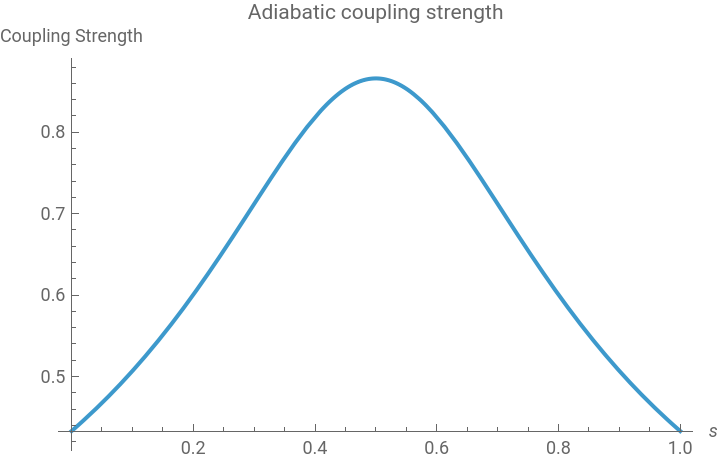
The max value of the coupling function is around s = 0.5, which makes sense as that is also when the ground state and first excited eigenstate are the closest as well.
Get the max value of the coupling.
Compute the minimum adiabatic time T.
Set the value of T to 5 times the minimum T necessary for the adiabatic condition to be satisfied:
System Evolution and Problem Results
System Evolution and Problem Results
Now, to solve the problem and actually run the adiabatic algorithm, the system needs to evolve through time. Internally, this involves solving the time-dependent Schrödinger equation with the Hamiltonian, but the framework has a QuantumEvolve function for the same purpose. The evolution starts from a uniform superposition, then evolve until time T with the Hamiltonian.
Extract all the probabilities associated with the 3rd basis state during the evolution:
Find the first time value at which a probability is greater than 0.99. Mark this on the plot if it exists, otherwise the value is set to 0 and isn’t shown on the plot:
Extract the probabilities of each basis state using ProbabilityList and plot them. The dotted line shows the first time the probability for state 10 is greater than 0.99:
Extract the eigenstate as a statevector:
Plot square of each element in the statevector to get probabilities:
Compute fidelity of evolution state at a specific timestep with marked state, then store results in a list:
Plot fidelity with marked state over evolution period:
The plot for fidelity very closely matches the path of the probability for the 01 state in the evolution graphs. This makes sense, because as the vector points more and more towards the 01 basis vector in 4-dimensional space, it becomes more and more similar to the target vector of 01 itself, causing the fidelity to follow a similar path.
Local Adiabatic Evolution
Local Adiabatic Evolution
Spectral Gap and Coupling Analysis
Spectral Gap and Coupling Analysis
Below, the same computation for the eigenvalues is done. The paper mentioned there will be N-2 degenerate eigenvalues of 1 alongside the actual eigenvalues, which are the ones with the square roots.
The plot shows the evolution over time of the energy levels. The s(t) function needs the minimum gap, so the symbolic gap between the eigenvalues is calculated and minimized.
Get ground state and first excited state energy levels:
Compute symbolic gap between the first excited state and ground state energy levels:
Minimize the symbolic gap between the two energy levels via NMinimize:
The coefficients of the term (-1 + s) (s) seem to form a sequence, so I extract them to analyze them:
Use the FindSequenceFunction to describe these coefficients with a sequence:
Using this sequence function, turn it back into a square root (as the terms were squared earlier), then put the n terms in terms of dimension N to get a clean formula for the minimum energy gap, g, over qubit counts:
Square each peak value to get rid of the square root, then use FindSequenceFunction to find a symbolic expression in terms of n describing the peaks:
Compute the limit as n goes to infinity:
Local Adiabatic Scheduling Enforcement
Local Adiabatic Scheduling Enforcement
Invert the result of the integration, making sure to apply Normal to get rid of the conditional expression that would otherwise be returned. I also use Function[] to assign parameter s to tExpr without using a pure anonymous function, as that would otherwise mess with the parameter of [t] and reduce code readability:
The error parameter epsilon is a heavy factor in controlling the adiabatic time T. I choose to set it 0.2 based off observation, as on average, it provides values for T that are long enough to ensure ample time for convergence to the correct basis state without wasting too much time.
Based on the chosen epsilon value, the time T can be calculated by plugging in s = 1 into t(s, epsilon), as it is required that s(T) = 1 which is the same thing as t(s = 1, epsilon) = T:
System Evolution and Problem Results
System Evolution and Problem Results
Now, the system is evolved with the Schrödinger equation to get the probability and fidelity results.
Create a function extract the probabilities of one basis state at one timestep:
Create a function to store probabilities for every basis state across the evolution period:
Compute the time value for which the probability of the third element basis state (the marked basis state) has a probability greater than 0.99 at any point. If it doesn’t exist, store 0:
Plot basis probabilities throughout evolution. The dotted line shows the first time the probability for state 10 is greater than 0.99:
Convert the time-dependent Hamiltonian into a QuantumState to extract the lowest energy eigenvector, then extract probabilities:
Sample time values across the evolution period, using Transpose to get every single probability for a basis state in its own list:
The evolution based on the ground state Eigenvector is much smoother compared to the NDSolveValue based solution. This could still be due to structural and numeric differences between eigenvector and Schrödinger-based evolution, as the resulting probabilities are still the same, reaching the solution faster than that of the baseline adiabatic algorithm.
I calculate fidelities in a similar way to what was done with the baseline adiabatic algorithm.
I calculate fidelities in a similar way to what was done with the baseline adiabatic algorithm.
Get all fidelities with QuantumSimilarity using a Table through a bunch of points:
Plot the fidelities over the time period:
Counterdiabatic Evolution
Counterdiabatic Evolution
Define the lambda scheduling function:
Adiabatic Gauge Potential Approximation
Adiabatic Gauge Potential Approximation
where
This works because each commutator in the series kind of acts like a derivative in a Taylor series would, so the higher order that the expansion is, the more that any diabatic excitations happen that could cause the system to leave the ground state. Within this summation, the alpha coefficients for each of the commutators are calculated by solving the linear system of equations:
This works because each commutator in the series kind of acts like a derivative in a Taylor series would, so the higher order that the expansion is, the more that any diabatic excitations happen that could cause the system to leave the ground state. Within this summation, the alpha coefficients for each of the commutators are calculated by solving the linear system of equations:
For each gamma term in the matrix for calculating the alpha coefficient, use the built in Norm function to calculate the Frobenius norm at order k:
Construct the full linear system to solve for the alpha coefficients. There are two iterators because the Gamma terms are slightly offset in the matrix and are even along the diagonal:
Construct the final AGP approximation at order l, timestep t, and total adiabatic time T:
At t = 0.5, the agpApproximation at different orders look oddly similar. This reveals something about the nature of the nested commutator approximation for the AGP: it is near static for this specific problem. I will also compute other diagnostics, like matrix rank and its eigenvalues, to inspect this further. Because of this, I will only be using order l = 1 for the rest of the AGP approximations in the counterdiabatic section.
Output the approximation for orders l = 1 and l = 2:
Calculate the rank (number of linearly independent columns) of the order 1 through 4 commutator matrices:
The ranks are all 2 because of the way they were constructed, since this Grover problem space collapses onto a 2x2 space due to the problem formulation. This has been hinted at by the N - 2 degenerate eigenvalues earlier along with the projector-based construction of the problem.
Output the eigenvalues for each of the approximations:
Notice that there are 2 degenerate eigenvalues and 2 actual ones. This matches the pattern seen earlier with N-2 degenerate eigenvalues, as the problem will always collapse onto 2 actual ones. This is consistent over all orders, too.
Evolution With Added Counterdiabatic Terms
Evolution With Added Counterdiabatic Terms
Compute the derivative of lambda symbolically:
Compute the total Hamiltonian adding the scaled AGP approximation to the adiabatic Hamiltonian:
T is set to 10, since there is no good analytical bound for what T should be after adding the CD driving terms due to the fact that they cancel out adiabatic transitions, so it is unnecessary to try deriving a bound for the adiabatic time.This has no negative effects in the results, so it is fine.
Use NDSolveValue to evolve the system:
Create a helper function to calculate the probability for a given statevector at timestep t in the evolution solution:
Get probabilities for all points in the range of T:
Separate the points into their own lists for plotting using All in part:
Plot probabilities throughout evolution period. The dotted line shows the first time the probability for state 10 is greater than 0.99:
Function to retrieve eigenvectors at time t of the total Hamiltonian using the parameter from QuantumOperator:
Get probabilities from eigenvectors at time t using ProbabilityList:
Get all points during eigenvector evolution and use Transpose to put each basis state probability into its own list:
Plot eigenvector based evolution over time:
I also analyze fidelity like before, using QuantumSimilarity between the current timestep in the NDSolveValue solution and the target quantum state, then plotting with ListLinePlot.
Retrieve fidelities by tabling through all solution points, then using QuantumSimilarity:
Plot state fidelity during evolution:
Results
Results
To compare the performance between all three methods, I create a combined fidelity plot and probability plot relative to each method’s time period.
This will involve retrieving all of the fidelity point lists from all three methods and finding their respective lengths. This is necessary as the length of each list is different, so plotting them as-is would make the plot incorrect. Instead, I extend the lists to be the same length for the plot to be accurate.
This will involve retrieving all of the fidelity point lists from all three methods and finding their respective lengths. This is necessary as the length of each list is different, so plotting them as-is would make the plot incorrect. Instead, I extend the lists to be the same length for the plot to be accurate.
Retrieve all fidelity point lists from the three methods:
Get the length of each of the fidelity lists to compare them:
Find the longest fidelity length (which will be of the baseline algorithm as it is the slowest):
Extend localFidelities and cdFidelities to the length of baselineFidelities by adding a ConstantArray with their last element to them:
Plot the fidelities of all three methods against each other over time:
Extract the third basis state points from each of the lists. BaselinePoints already has the third basis state points inside, so that is used as-is:
Get the length of each of the lists:
Find the max length of the probability list (which will be the baseline probabilities):
Extend the basisLocalPoints and basisCdPoints lists to be the same length as the baselinePoints:
There is a clear speed difference between the three methods, with baseline being the slowest as expected, followed by the local adiabatic method then the counterdiabatic method.
Conclusion
Conclusion
This work compares three types of adiabatic quantum algorithms on Grover’s search problem. I analyzed the spectral gap between ground state and excited state Hamiltonian eigenstates to determine the minimum adiabatic time necessary for the algorithm to be successful, found an analytic formula for the adiabatic coupling given an N-dimensional quantum system, evolved Hamiltonians via the time-dependent Schrödinger equation, computed probability and fidelity metrics, and plotted results amongst the algorithms against each other. Counterdiabatic driving offered a large speedup in terms of probability measurement and fidelity, but also encountered some issues with the computation of the adiabatic gauge potential. The local adiabatic search also performed better than the baseline adiabatic algorithm due to its better enforcement of the adiabatic condition, but still worse than counterdiabatic driving.
Limitations
Limitations
One of the largest limitations across the results of this project was the basis of choosing the time T. For the local adiabatic search, the time relied entirely on the parameter epsilon, which was almost entirely an arbitrary choice. The T value for the baseline adiabatic algorithm was also arbitrary as well, as although there was a minimum time T available, T needed to be much larger than that time anyways. For the counterdiabatic time, there was no indication of what the time should be at all, so it was set to 10 seconds without much reasoning. Including an optimization to find the minimum time T (or parameter epsilon) that would lead to adiabatic behavior would be a much more consistent basis for comparison between the three algorithms. Aside from this, the Grover problem structure limiting the AGP approximation to order l=1 along with making the exact AGP calculation impossible was also problematic, as it constrained the performance of the counterdiabatic method. Finally, the projector-based Grover problem setup itself is only one of many possible formulations of this problem, so testing other search formulations could possibly lead to more faborable behavior across these three algorithms.
Future Directions
Future Directions
The counterdiabatic search shows promise in future applications of quantum algorithms, however the approximation for the adiabatic gauge potential term is still problematic due to the nested commutator order not affecting the matrix. Working on a mathematical description of the Grover problem space and why the approximation is limited would allow a better understanding of how to improve the CD driving terms along with the approximation. Additionally, computing the exact adiabatic gauge potential term and analyzing the error between it and the approximation would help suppress nonadiabatic transitions much more effectively. Other than the AGP term, testing out different lambda scheduling functions and understanding effects of using trigonometric vs. polynomial functions could help with the enforcement of the adiabatic condition in the algorithm as well. Finally, optimizing for the minimum time necessary to preserve adiabatic transitions in the algorithms would allow for much more robust and exact estimates of the runtime on the algorithms.
References
References
◼
Adiabatic Gauge Potential in Quantum Systems. (2025). Emergentmind. https://www.emergentmind.com/topics/adiabatic-gauge-potential-agp
◼
Born, M., & Fock, V. (1928). Beweis des Adiabatensatzes. Zeitschrift F�R Physik, 51(3–4), 165–180. https://doi.org/10.1007/bf01343193
◼
Claeys, P. W., Pandey, M., Dries, S., & Polkovnikov, A. (2019). Floquet-engineering counterdiabatic protocols in quantum many-body systems [Review of Floquet-engineering counterdiabatic protocols in quantum many-body systems]. arXiv.Org. https://doi.org/10.1103/PhysRevLett.123.090602
◼
Farhi, E., Goldstone, J., Gutmann, S., & Sipser, M. (2000, January 28). Quantum Computation by Adiabatic Evolution. arXiv.Org. https://arxiv.org/abs/quant-ph/0001106
◼
Huerta-Ruiz, R., Araya-Gaete, M., Tancara, D., Solano, E., Barraza, N., & Albarrán-Arriagada, F. (2025). Quantum coherence and counterdiabatic quantum computing. arXiv.Org. https://arxiv.org/abs/2504.17642
◼
Roland, J., & Cerf, N. J. (2002). Quantum search by local adiabatic evolution. Physical Review A, 65(4). https://doi.org/10.1103/physreva.65.042308
Acknowledgements
Acknowledgements
I would like to thank my mentor Sebastian Rodriguez, and the teaching assistants that helped me edit this work Amrita Kumar and Daniel Xu. I would also like to thank my TA Hendry Xu for his guidance throughout the program, and my TA group for making my experience truly enjoyable and memorable while working on this project. Finally, I would like to thank the directors of the Wolfram Summer Research Program, Rory Foulger, Eryn Gillam, and Megan Davis alongside the CEO of Wolfram Research, Stephen Wolfram for helping me formalize my own ideas and publish this work.
Additional thanks to Stephen Wolfram for suggesting this project.
CITE THIS NOTEBOOK
CITE THIS NOTEBOOK
Accelerating adiabatic quantum algorithms on Grover's search with counterdiabatic driving
by Atharv Kanchi
Wolfram Community, STAFF PICKS, July 9, 2026
https://community.wolfram.com/groups/-/m/t/3749606
by Atharv Kanchi
Wolfram Community, STAFF PICKS, July 9, 2026
https://community.wolfram.com/groups/-/m/t/3749606