Wolfram Cloud Document

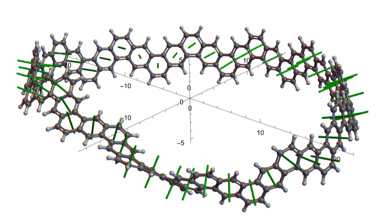
As Jason Biggs recently noted in his contribution “Overview of Wolfram Chemistry” on YouTube it might be interesting to see the normal vector of each benzene ring as you rotate the Möbius strip-like molecule around the z-axis.

Prerequisites...

For RingPattern[]

PacletInstall["WolframChemistry/ChemistryFunctions"]

Out[]=

PacletObject

Name: WolframChemistry/ChemistryFunctions

Version: 1.0.2



In[]:=

Needs["WolframChemistry`ChemistryFunctions`"]

Import of XYZ file
XYZ can be found attached to this post and also in https://static-content.springer.com/esm/art%3A10.1038%2Fs44160-022-00075-8/MediaObjects/44160_2022_75_MOESM3_ESM.txt (lines 1648 up to 1950)

In[]:=

nanobelt=Import["Möbius carbon nanobelt.xyz"]

Out[]=

Molecule

Formula:

200

100

Atoms: 300 Bonds: 350



Visualization

In[]:=

rings=FindMoleculeSubstructure[nanobelt,RingPattern[6],All]

Out[]=

{11,22,37,46,55,64,11,24,33,4198,5199,6200,16,27,39,48,513,611,110,211,313,412,517,615,114,215,317,416,521,619,116,218,323,422,520,621,122,227,329,424,525,623,126,227,329,428,533,631,130,231,333,432,537,635,132,234,339,438,536,637,138,243,345,440,541,639,142,243,345,444,549,647,146,247,349,448,553,651,148,250,355,454,552,653,154,259,361,456,557,655,158,259,361,460,565,663,162,263,365,464,569,667,164,266,371,470,568,669,170,275,377,472,573,671,174,275,377,476,581,679,178,279,381,480,585,683,180,282,387,486,584,685,186,291,393,488,589,687,190,291,393,492,597,695,194,295,397,496,5101,699,196,2101,3100,4102,5103,698,1102,2105,3109,4107,5104,6103,1105,2106,3111,4110,5108,6109,1110,2115,3117,4112,5113,6111,1114,2115,3117,4116,5121,6119,1118,2119,3121,4120,5125,6123,1120,2122,3127,4126,5124,6125,1126,2131,3133,4128,5129,6127,1130,2131,3133,4132,5137,6135,1134,2135,3137,4136,5141,6139,1136,2138,3143,4142,5140,6141,1142,2147,3149,4144,5145,6143,1146,2147,3149,4148,5153,6151,1150,2151,3153,4152,5157,6155,1152,2154,3159,4158,5156,6157,1158,2163,3165,4160,5161,6159,1162,2163,3165,4164,5169,6167,1166,2167,3169,4168,5173,6171,1168,2170,3175,4174,5172,6173,1174,2179,3181,4176,5177,6175,1178,2179,3181,4180,5185,6183,1182,2183,3185,4184,5189,6187,1184,2189,3188,4190,5191,6186,1190,2195,3197,4192,5193,6191,1194,2199,3200,4196,5197,6195}

In[]:=

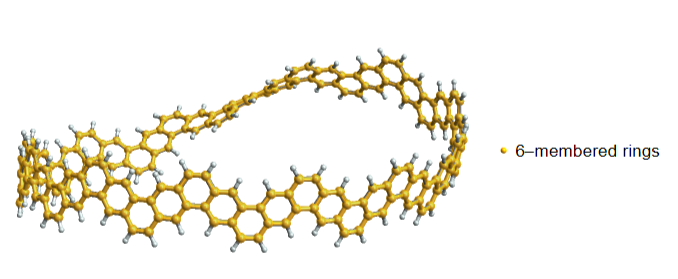
MoleculePlot3D[nanobelt,<|"6–membered rings"->RingPattern[6]|>,SphericalRegion->True]

In[]:=

ac=QuantityMagnitude[nanobelt["AtomCoordinates"]];

None of the 50 benzene rings are planar!

Or@@(CoplanarPoints[ac[[Values[#]]]]&/@rings)

Out[]=

False

Instead of complete 6 - membered rings, I just took every second atom, yielding 50 triangles

In[]:=

coords=ac[[#]]&/@Values[rings][[All,{1,3,5}]];Length[%]

Out[]=

Calculation of the center points for all triangles

In[]:=

cp=RegionCentroid[Triangle[#]]&/@coords

Out[]=

{{-0.0781133,14.7808,0.0000443333},{2.23021,14.7132,-0.879604},{-2.40342,14.6997,0.855405},{-4.35187,14.3229,-0.612281},{-6.24203,13.7002,-2.07522},{-8.44071,13.1092,-1.14179},{-10.598,12.3384,-0.19758},{-12.2195,11.0063,-1.49586},{-13.6789,9.45324,-2.74319},{-15.4322,8.16192,-1.59965},{-17.009,6.68177,-0.396219},{-17.8288,4.56335,-1.35575},{-18.3673,2.32408,-2.2438},{-19.0623,0.510532,-0.739163},{-19.3758,-1.3634,0.837714},{-18.9255,-3.69899,0.199691},{-18.1667,-5.96292,-0.426965},{-17.1873,-7.4486,1.25974},{-15.7649,-8.66673,2.8571},{-14.1947,-10.4166,2.1328},{-12.4949,-12.021,1.32958},{-10.2677,-12.0636,2.34267},{-7.92075,-11.7067,2.98373},{-6.05565,-12.9153,1.92902},{-4.15423,-14.1422,0.934006},{-1.98453,-13.0501,0.619579},{0.0772853,-11.8788,-0.052782},{2.13548,-13.0639,-0.663968},{4.35467,-14.1112,-0.937645},{6.24289,-12.9121,-1.95626},{8.09856,-11.7006,-3.0371},{10.4192,-12.0313,-2.33231},{12.6535,-11.9121,-1.29871},{14.3543,-10.3207,-2.08891},{15.9116,-8.55961,-2.82987},{17.2747,-7.33314,-1.20482},{18.224,-5.7898,0.471929},{18.9649,-3.52061,-0.13368},{19.3919,-1.18541,-0.797588},{19.0382,0.655938,0.787804},{18.3096,2.49948,2.26897},{17.7388,4.73343,1.39531},{16.9047,6.83361,0.405689},{15.3257,8.27319,1.62268},{13.542,9.58052,2.74044},{12.0542,11.1139,1.50624},{10.4319,12.4204,0.181121},{8.29503,13.165,1.14731},{6.06623,13.7614,2.05434},{4.15717,14.3584,0.608279}}

The normals as tubes, each tube extends over both sides of the triangle planes

In[]:=

normalLines[cp_,coords_]:=Module[{cross},cross=Cross[Sequence@@(cp-#&/@coords[[;;2]])];Tube[{cp+cross,cp-cross},0.1]]

In[]:=

nl=MapThread[normalLines[#1,#2]&,{cp,coords}];

In[]:=

Show[Graphics3D[{Red,Point[cp],Darker[Green],nl}],MoleculePlot3D[nanobelt],AxesTrue,BoxedFalse,AxesOrigin->{0,0,0},SphericalRegion->True]

ListAnimate and Animate graphics

In[]:=

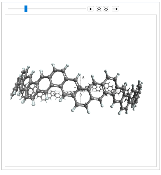
rotGr=Table[MoleculePlot3D[nanobelt,SphericalRegion->True,AxesTrue,BoxedFalse,AxesOrigin->{0,0,0},ViewVector{25Cos[t],25Sin[t],0}],{t,0,2Pi,0.05}];

In[]:=

ListAnimate[rotGr,DisplayAllSteps->True]

For control purposes, the ViewVector as red lines

For some reason, I had to swap the first two coordinates ...

Adjusted ViewVector; interpolation for a smoothed “tracking shot”

Final animation

Export the animation as mp4 file

Produce an animated gif

CITE THIS NOTEBOOK

Visualization of a Möbius carbon nanobelt and normal vectors on all benzene rings
by Armin Vollmer
Wolfram Community, STAFF PICKS, August 3, 2023
https://community.wolfram.com/groups/-/m/t/2982851