ABSTRACT (original article): In schedulability analysis, the timing of all tasks of a real-time system is verified by finding the worst-case behavior. Two well-studied methods in this field are the demand bound test and the real-time calculus. However, the former is only applicable to specific task models whereas the latter does not formalize concrete task models of complex job patterns. This work presents a new approach to formally describe and analyze the worst-case of any complex job pattern. The approach consists of a task model that reduces all kinds of job patterns to a vector space of jobs. Furthermore, the worst-case analysis searches for local maxima to find the worst-case of any job pattern by differentiating any cumulative function of the real-time calculus. Therefore, the analysis in this work implies an algorithm to compute request as well as demand bounds by construction. This formal approach allows the integration of mathematical results from real-time calculus into real-time scheduling theory. In fact, this is, to our knowledge, the first method to compute a demand bound function with arbitrary deadlines by a min-plus deconvolution in the real-time calculus. This now allows the analysis of complex task models as the generalized multiframe model in the real-time calculus. CITATION (original article): Iwan Feras Fattohi, Christian Prehofer, Frank Slomka, A novel real-time calculus for arbitrary job patterns and deadlines. Journal of Systems Architecture, 155 (2024), 103248. https://doi.org/10.1016/j.sysarc.2024.103248
Introduction
Introduction
Schedulability analysis is applied in the field of embedded real-time systems. A real-time system is a computing system that is characterized by software tasks that must complete their execution within a given time duration, called the deadline [1]. Two well-known methods to check whether deadlines are always met are the response time analysis [2] and the demand bound test [3]. The former computes the maximum response time that a task can ever achieve which is then compared to the deadline, whereas the latter compares the utilization of the whole set of tasks against the deadline.
The schedulability analysis problem is known to be NP-hard. Therefore, the literature focusses on the development of computationally efficient algorithms for special instances of this problem. To this end, one can restrict the timing behavior of tasks. The first task model is introduced by Liu & Layland [4] in which the timing behavior is described by three parameters. The first is the worst-case execution time (WCET) of a task which describes the maximum execution time that the program of the task requires on a specific hardware. The second parameter is the deadline that specifies a time duration in which the task must finish execution. The time duration from the start to the completion of the execution of the task is called the response time. If the response time of the task is greater than the deadline, then the correct functionality of the computing system is not guaranteed anymore. Note that the response time of the task is greater or equal to its execution time if the given scheduling policy allows task preemption. The third parameter is the period of the task which describes that the task is periodically requested for execution. The periodic request can be induced by an external event from the physical environment of the embedded system. A typical application is the periodic sampling of a controller in control engineering.
In the Liu & Layland model, every instance of the task, that is called a job, has the same WCET and deadline. Furthermore, the time distance among all jobs is equal to the period of the task. The time point at which a task is requested for execution upon which a job is generated is called the request time. Since Liu & Layland, this task model has been refined to allow periodic and non-periodic patterns among the WCET, deadline and time distance between jobs as well. This means the literature on schedulability analysis consists of many different task models. If an embedded system designer wants to apply a schedulability analysis to a task set, the designer has to find at first the right task model in the literature for that task set. To avoid the situation that none of the known task models are applicable to the given task set, a general task model is required. By general, we mean that a task model has to be able to describe any kind of timing behavior of tasks. Particularly, a task model is needed that allows any pattern of request times, WCETs and deadlines of jobs.
Our work formalizes any timing pattern of jobs as a linear combination of jobs. More precisely, any kind of timing pattern among the request times, WCETs and deadlines of jobs is represented as a linear combination in a vector space of jobs. Any known task model from the literature can be shown to be a vector subspace. To formulate such a vector space, we need at first a mathematical model of a job. Slomka and Sadeghi [5] are the first ones to apply the Dirac Delta to describe a task request in a real-time system. The idea is that the request of a task occurs instantaneously at a given time point. As an example, a periodic event that causes a task to be periodically requested for execution can the described by a Dirac comb. A request causes a state change of the task as it becomes ready for execution. The state change can be in turn described by a Heaviside step function. Briefly said, the Dirac delta and the Heaviside function are the mathematical foundation of our task model for schedulability analysis.
Model
Model
Our idea is to formalize a job by a scaled and shifted Dirac Delta:
In[]:=
job[t_,s_,c_]:=c*DiracDelta[t-s]
where t represents time, s represents the request time of the job and c represents the WCET of the job. Hence, the request time of the job is described by the shift s of the Dirac delta and the WCET is formalized by the scaling factor c of the Dirac delta.
In[]:=
job[t,s,c]
Out[]=
cDiracDelta[-s+t]
For example, a job that is requested at time point s = 5 with a WCET (or also called computational workload) of c = 3 is represented by
In[]:=
job[t,5,3]
Out[]=
3DiracDelta[-5+t]
The novelty of this model is that we can directly calculate on jobs by using known calculation rules of the Dirac delta that were originally introduced by Paul Dirac [6]. For example, to calculate the computational workload that is requested in a given time interval [a,b], we integrate the Dirac delta over [a,b]. The resulting expression of the integral depends on the relation between the interval boundary a and b to the request time s. Some of the cases are:
Integrate[job[t,s,c],{t,a,b},Assumptions->a<s<b]Integrate[job[t,s,c],{t,a,b},Assumptions->s<a<b]Integrate[job[t,s,c],{t,a,b},Assumptions->a<b<s]
Out[]=
c
Out[]=
0
Out[]=
0
so that the workload of the job is counted if a < s < b, i.e. if the job is requested inside the open interval (a,b). If the job is requested outside of the closed interval [a,b], its workload is not counted. The integral of the Dirac delta is therefore a method to calculate computational workload in a given time interval which is essential in calculating the utilization of a task set or the response time of a task. The corner cases s = a, s = b or a = s = b result in expressions dependent on the Heaviside function:
In[]:=
Integrate[job[t,s,c],{t,a,b},Assumptions->a<=s<b]Integrate[job[t,s,c],{t,a,b},Assumptions->a<=s<=b]
Out[]=
cHeavisideTheta[-a+s]
Out[]=
c(-1+2HeavisideTheta[-a+b])HeavisideTheta[s-bHeavisideTheta[a-b]-aHeavisideTheta[-a+b]]HeavisideTheta[-s+aHeavisideTheta[a-b]+bHeavisideTheta[-a+b]]
where the first expression c HeavisideTheta[-a+s] results in c HeavisideTheta[0] if s = a:
In[]:=
Integrate[job[t,s,c],{t,a,b},Assumptions->a==s<b]
Out[]=
cHeavisideTheta[0]
so that it is open to decide whether to count workload if the request of the job occurs at the interval boundary a. The same case occurs if s = b holds. This means HeavisideTheta[0] represents that it open to decide whether to count the workload of a job if it occurs at an interval boundary. If we decide to define HeavisideTheta[0] = 1, then we count workload at interval boundaries and with HeavisideTheta[0] = 0 we exclude workload at interval boundaries. We therefore obtain a mathematical model to describe the in- or exclusion of workload at interval boundaries. The expression
In[]:=
Integrate[job[t,s,c],{t,a,b},Assumptions->a<=s<=b]
Out[]=
c(-1+2HeavisideTheta[-a+b])HeavisideTheta[s-bHeavisideTheta[a-b]-aHeavisideTheta[-a+b]]HeavisideTheta[-s+aHeavisideTheta[a-b]+bHeavisideTheta[-a+b]]
models all kinds of cases among s, a and b. For example, if a < b, then the last term simplifies to
In[]:=
Assuming[a<b,Refine[c(-1+2HeavisideTheta[-a+b])HeavisideTheta[s-bHeavisideTheta[a-b]-aHeavisideTheta[-a+b]]HeavisideTheta[-s+aHeavisideTheta[a-b]+bHeavisideTheta[-a+b]]]]
Out[]=
cHeavisideTheta[b-s]HeavisideTheta[-a+s]
which is a rectangular function, that we call the Heaviside mask since it returns c if the request occurs inside the interval [a,b]. For example, if c = 2, a = 1 and b = 3, we get
In[]:=
heavisideMask[s_,a_,b_]:=HeavisideTheta[b-s]HeavisideTheta[s-a]Plot[2heavisideMask[s,1,3],{s,-1,4},ExclusionsStyle->Dashed,AxesLabel->{"t","workload"}]//AbsoluteTimingPlot[Integrate[job[t,s,2],{t,1,3}],{s,-1,4},ExclusionsStyle->Dashed,AxesLabel->{"t","workload"}]//AbsoluteTiming
Out[]=
0.274359,
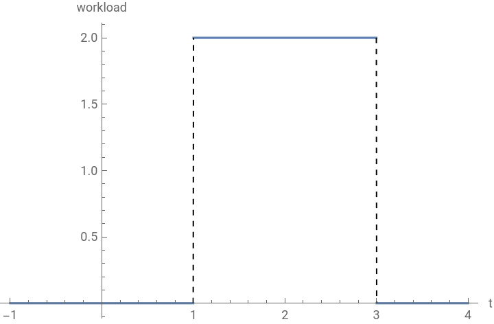
Out[]=
2.04826,
so that we can either calculate the workload of a job in a given time interval using the integral or by using the Heaviside mask which has a shorter runtime.
Until now, we only calculated on a single job. The vector space of jobs and hence the calculation of the workload of any kind of linear combination of jobs, called a job train, is formalized by a summation of scaled and shifted Dirac impulses:
In[]:=
jobTrain[t_,shifts_,workloads_,degree_]:=Sum[job[t,shifts[[n]],workloads[[n]]],{n,1,degree}]
where shifts and workloads are lists of request times and WCETs of all jobs and degree is the number of jobs. The function jobTrain represents a general linear combination in the vector space of jobs. Vector addition is the addition of Dirac deltas and scalar multiplication is the scaling of Dirac deltas. For example, a job train of 5 jobs is given by
In[]:=
shifts1={1,5,13,21,27};workloads1={3,2,4,1,5};degree1=5;jobTrain[t,shifts1,workloads1,degree1]
Out[]=
5DiracDelta[-27+t]+DiracDelta[-21+t]+4DiracDelta[-13+t]+2DiracDelta[-5+t]+3DiracDelta[-1+t]
We can add another job train and also scale the result:
In[]:=
shifts2={-5,-1,4,9};workloads2={3,1,2,5};degree2=4;scalar1=3;scalar1*(jobTrain[t,shifts1,workloads1,degree1]+jobTrain[t,shifts2,workloads2,degree2])
Out[]=
3(5DiracDelta[-27+t]+DiracDelta[-21+t]+4DiracDelta[-13+t]+5DiracDelta[-9+t]+2DiracDelta[-5+t]+2DiracDelta[-4+t]+3DiracDelta[-1+t]+DiracDelta[1+t]+3DiracDelta[5+t])
Note that the shift can be any real number and the workload can be any positive real number. The function jobTrain is applicable to any task since it only assumes a job train to be given. More precisely, our model only assumes that a task generates a sequence of jobs and it does not assume that these jobs are generated according to a specific pattern. By also showing that the function jobTrain spans a vector space, it follows that any task model can be described by our model.
We can also describe well-known task models from the literature. These models typically describe periodic tasks. A job of a job train can be modified to occur periodically by the convolution of the job with a Dirac comb(see [7] for the complete formalization). This simply means that a job that occurs at time point s is replicated every p time points:
We can also describe well-known task models from the literature. These models typically describe periodic tasks. A job of a job train can be modified to occur periodically by the convolution of the job with a Dirac comb(see [7] for the complete formalization). This simply means that a job that occurs at time point s is replicated every p time points:
In[]:=
Convolve[Sum[DiracDelta[t-n*p],{n,0,3}],job[t,s,c],t,x]
Out[]=
c(DiracDelta[p+s-x]+DiracDelta[2p+s-x]+DiracDelta[3p+s-x]+DiracDelta[-s+x])
But the convolution of two Dirac deltas implies that the one Dirac impulse is shifted by the shift of the other Dirac impulse (see [7]). Hence, we can replace convolution by subtraction:
In[]:=
Sum[job[t,s+n*p,c],{n,0,3}]
Out[]=
cDiracDelta[p+s-t]+cDiracDelta[-s+t]+cDiracDelta[-3p-s+t]+cDiracDelta[-2p-s+t]
Regarding the literature, this series of Dirac deltas describes a periodic task with offset s, period p and WCET c that generates 4 jobs as n goes from 0 to 3. In the literature, the task models usually account for infinitely many jobs [8]:
In[]:=
jobTrainOffset[t_,s_,c_,p_,degree_]:=Sum[job[t,s+n*p,c],{n,0,degree}]
The summation of finitely many job trains of periodic tasks with offsets that all have the same period p results in a job train of a generalized multiframe task [9]:
In[]:=
jobTrainGMF[t_,shifts_,workloads_,p_,numFrames_,degrees_]:=Sum[Sum[job[t,shifts[[m]]+n*p,workloads[[m]]],{n,0,degrees[[m]]}],{m,1,numFrames}]
Note that the periodic task with offset and the GMF are originally defined to generate infinitely many jobs, so that we have to set degree = Infinity to describe their infinite job trains. To calculate the computational workload of an arbitrarily constructed job train, we apply the integral again. Due to the linearity of the integral, the integral of a job train is equal to the summation of the integral of each individual job. But this means that we can calculate on Heaviside masks as well (a formal proof of this equivalence is given by [7]):
In[]:=
a=-10;b=13;Integrate[jobTrain[t,shifts1,workloads1,degree1],{t,a,b}]//AbsoluteTimingSum[Integrate[job[t,shifts1[[n]],workloads1[[n]]],{t,a,b}],{n,1,degree1}]//AbsoluteTimingSum[workloads1[[n]]*heavisideMask[shifts1[[n]],a,b],{n,1,degree1}]//AbsoluteTiming
Out[]=
{0.062645,5+4HeavisideTheta[0]}
Out[]=
{0.053778,5+4HeavisideTheta[0]}
Out[]=
{0.000042,5+4HeavisideTheta[0]}
so that we define the requestLoad as a function that computes the workload of all jobs in a given time interval [a,b]:
In[]:=
requestLoad[shifts_,workloads_,degree_,a_,b_]:=Sum[workloads[[n]]*heavisideMask[shifts[[n]],a,b],{n,1,degree}]
The function requestLoad computes the sum of the workloads of all jobs that are requested in the time interval [a,b] while returning HeavisideTheta(0) if a job occurs at the boundaries a or b. If a job train is given, then requestLoad is a two-dimensional function of the interval boundaries a and b. If a is constant and b is increasing, then requestLoad is a monotonically increasing function:
In[]:=
a=-2Plot[requestLoad[shifts1,workloads1,degree1,a,b],{b,a,40},ExclusionsStyle->Dashed,AxesLabel->{"b","requestLoad(-2,b)"}]
Out[]=
-2
Out[]=
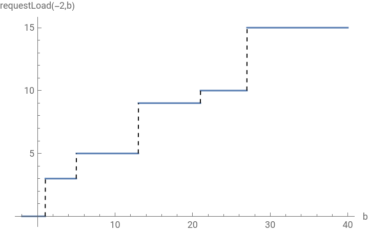
If both a and b are increasing such that b - a is constant, then the function requestLoad can increase and decrease . More precisely, a window of a constant time duration b - a is shifted over time and calculates the amount of workload in the current interval[a, b] :
In[]:=
a=3;b=10;Plot[requestLoad[shifts1,workloads1,degree1,t+a,t+b],{t,-10,30},ExclusionsStyle->Dashed,AxesLabel->{"t","requestLoad(t + 3, t + 10)"}]
Out[]=
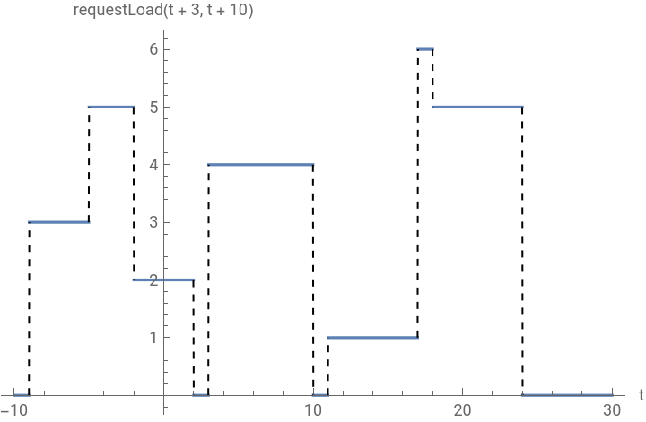
We can see that the maximum of the request load is 6. This means the maximum workload of all jobs that can be found in any time interval of duration t + b -(t+ a) = b - a = 7 is equal to 6 which is found between t = 17 and t = 18.
Therefore, if we keep the interval duration of the request load constant, we can investigate the maximum amount of workload for a certain interval duration which is in schedulability analysis the basis for a utilization-based test. Let us define this special requestLoad as the deltaRequestLoad as it is bounded from above:
Therefore, if we keep the interval duration of the request load constant, we can investigate the maximum amount of workload for a certain interval duration which is in schedulability analysis the basis for a utilization-based test. Let us define this special requestLoad as the deltaRequestLoad as it is bounded from above:
For the familiar reader, the last two plots represent a min-plus self-deconvolution of the deltaRequestLoad for the interval duration Δ = b - a = 7. The min-plus self-deconvolution is a well-known operator of the network calculus [10] which is applied in the real-time calculus to determine arrival curves. To calculate the request load for a periodic task model we can apply the integral to their periodic job trains as well, since we know by the vector space property that these job trains are special linear combinations in the vector space of jobs. For example, we can calculate the request load of a GMF task in the interval [-10,100] as follows:
The integral can be distributed over the three summation. Then, the integral and the infinite series can be swapped by Fubini’s theorem since the integral of the given infinite series is finite (see [5]). Then, we substitute the integral of a series of Dirac deltas by a series of Heaviside masks and obtain the request load of periodic tasks:
so that we can see in the first plot the periodic increase and decrease by a value of 4 which is characteristic for a periodic task with offset. Whereas for the GMF task, a periodic repetition is seen after all four frames have been cycled through. Note that the run time of the Plot function is impacted by the evaluation of an infinite series of Dirac deltas. We can speed up the evaluation by bounding the infinite series from above. In case of a GMF task, we know that the highest job index n, such that the n-th job is counted as request load is t + Δ ≥ s + n*p which means (t + Δ - s) / p ≥ n so that n is upper bounded by Ceiling[(t + Δ - s) / p]:
Schedulability Analysis - The Demand Bound Test
Schedulability Analysis - The Demand Bound Test
After the discussion of request loads which are fundamental to analyze the utilization and the response time of a tasks, we introduce the demand load. The demand load of a job adds another condition for the workload of a job to be counted in a given time interval. To describe the demand of a job, we define the absolute deadline D which is the time point until which the job must have completed execution. Additionally, we define d = D - s as the relative deadline of a job which in turn describes the time duration between the absolute deadline and the request time of the job. As originally defined by Baruah et al. [3], a job has a demand of workload c in the time interval [a,b] if its request time s as well as its absolute deadline D occur within the closed interval [a,b]. We can translate these conditions under which workload is counted using Heaviside functions:
The functions heavisideUpper and heavisideLower describe the right- and left-continuous Heaviside function. the function heavisideDemandMask represents a Heaviside mask that returns one if the request time s and the absolute deadline D of a job occur within the interval [a,b]. The result of the mask at the corner cases s = a or D = b depends on which Heaviside functions are applied as heavisideLeft and heavisideRight. For example, consider a job requested at time point s = 5 with an absolute deadline at time point 8. Furthermore, consider the time interval [a,b] = [4,8]. Then, the heavisideDemandMask returns the following values dependent on the chosen Heaviside function:
where heavisideDemandMask[5, 8, 4, 8, heavisideUpper, heavisideUpper] represents a Heaviside mask of the closed interval [4,8], so that the absolute deadline at time point D = 8 = b is also included, hence the function returns 1. Contrary, heavisideDemandMask[5,8,4,8,heavisideUpper,heavisideLower] returns 0 since the Heaviside mask considers the right-open interval [4,8), so that the absolute deadline of D = 8 results in heavisideLower[b - D] = heavisideLower[8 - 8] = 0 and hence the job has a demand of 0 for the given Heaviside mask. If we apply HeavisideTheta, then we get HeavisideTheta[b - D] = HeavisideTheta[8 - 8] = HeavisideTheta[0] as the last output shows, so that it is yet open to decide whether to include the absolute deadline and hence to decide whether the job has a demand greater than 0 for the given heavisideDemandMask. Based on the heavisideDemandMask, we can now formulate the demandLoad of a jobTrain:
The demandLoad implicitly provides a schedulability test that is originally introduced by Baruah et al. Particularly, if the demandLoad for a given time duration Δ is greater than Δ, then at least one of the tasks will have a response time greater than its relative deadline, so that the task will miss its deadline and therefore the task set is not schedulable. The reason is that the demandLoad accumulates the workload of all jobs that are requested and must be completed in a given time interval [t, t + Δ]. That means all of these jobs cannot be executed before t, since they are requested at or later than t. Furthermore, they all must complete execution before t + Δ. Assume that all jobs contributing to the demand load in the interval [t, t + Δ] are requested at the earliest possible time point, which is t, and must all be completed at the latest possible time point, which is t + Δ. Then, if the demandLoad in [t, t + Δ] is equal to Δ + ϵ for some ϵ > 0, then at least one of the jobs contributing to this demandLoad will be completed at t + Δ + ϵ, so that this job will miss its deadlines since its deadline is at or before t + Δ by the definition of the demandLoad. Note that during this discussion, no assumption is made on the execution order of the jobs, so that the schedulability analysis based on the demand load is independent from the chosen scheduling policy. For more technical details, see Baruah[3], Buttazzo [1], or also our paper [11].
Let us visualize the schedulability analysis based on an example.
Let us visualize the schedulability analysis based on an example.
Consider a jobTrain of two jobs that is specified by the following request times, workloads and absolute deadlines:
Then, we can demonstrate the schedulability analysis for the interval duration Δ = 10 and a heavisideDemandMask for a closed interval as follows:
The orange constant represents the interval duration Δ = 10. If the demandLoad exceeds the orange bound, then at least one of the two jobs will miss its deadline for any execution order of the jobs. Between t = 0 and t = 1, we can see that the demandLoad exceeds the orange bound, so that the given jobTrain is not schedulable.
As Δ is a non-negative real number and t is a real number, the schedulability analysis would have to check infinitely many t and Δ. Therefore, the literature on this so-called demand bound test proposes algorithms that reduce the infinitely many to a finite set of test points. However, the proposed algorithms assume certain task models. Our approach is to provide an algorithm that is applicable to any task model, i.e. to any kind of jobTrain with arbitrary patterns regarding request times, workloads and deadlines. To illustrate our idea, let us analyze the two-dimensional demandLoad function dependent on t and Δ independently. To this end, we apply the demandLoad function of a GMF task. Furthermore, we apply the GMF task example of [9].
As Δ is a non-negative real number and t is a real number, the schedulability analysis would have to check infinitely many t and Δ. Therefore, the literature on this so-called demand bound test proposes algorithms that reduce the infinitely many to a finite set of test points. However, the proposed algorithms assume certain task models. Our approach is to provide an algorithm that is applicable to any task model, i.e. to any kind of jobTrain with arbitrary patterns regarding request times, workloads and deadlines. To illustrate our idea, let us analyze the two-dimensional demandLoad function dependent on t and Δ independently. To this end, we apply the demandLoad function of a GMF task. Furthermore, we apply the GMF task example of [9].
We can see that if we keep t constant and increase Δ, we obtain a periodic function that is monotonically increasing whereas if we keep Δ constant and increase t, we obtain a function that has a maximum. A combination of both of these properties can be seen in a 3D plot of the demandLoad function:
The 3DPlot shows in direction of Δ the monotonically increasing demand load and in direction of t the bounded demand load. The fat black curve represents the 2D plot of the demand load for Δ = 22. Our approach is to determine a function of Δ that calculates for the given interval duration Δ the maximum demand load. The reason is that a simple schedulability analysis is to test whether the maximum is greater than Δ because then there exists at least one time point t, such that some job will miss its deadline. The maximum demand load is also known as the demand bound in the literature. Therefore, in the following, we present the computation of the so-called demand bound function for any kind of job and deadline pattern. This means, for any kind of job train, we have to find the maximum demand load for a given interval duration Δ. In classical calculus, a continuous function attains a global maximum and minimum in a closed interval. We call the interval in which we search the maximum the analysis interval [t_B, t_E]. In the literature of schedulability analysis, the analysis interval is usually determined based on the periods of the tasks, because if multiple periods of the tasks are considered in the analysis interval, then it is ensured that the maximum has occurred at least once.
To illustrate the analysis of the demand bound, we wrote our own plot function that allows to highlight function values at time points at which jump discontinuities occur.
To illustrate the analysis of the demand bound, we wrote our own plot function that allows to highlight function values at time points at which jump discontinuities occur.
For example, if we define an analysis interval of [-6,28] for the GMF task, we can visualize the search space for the maximum dependent on different heavisideDemandMasks using plotLoadFunction:
The plots show the demandLoad function for four different Heaviside masks. We can see that the choice of the Heaviside mask changes the function value at jump discontinuities. We can see by the example that including multiple periods of the task in the analysis interval [t_B, t_E] ensures to find the maximum demand load. If periods are not given, we can still define an analysis interval and search for the maximum. However, it is not guaranteed that the maximum for the given analysis interval is the highest value of the demand load for all possible analysis intervals. Our approach in finding the maximum for a given analysis interval is to determine all time points t at which local maxima are found. As the demandLoad is a piece-wise constant function, it follows that a local maximum is found after a discontinuous increase of the function. Furthermore, if two or more discontinuous increasings occur consecutively without a decrease in between, see t = -20 to t = 0 in the plot, then we only have to consider the last increase to find a local maximum. In the example this means from all time points in the interval [-20, 0] we have to select one time point of the interval [-5,0]. Therefore, for a given analysis interval [t_B, t_E], we obtain a finite set of time points t that give rise to local maxima of the demandLoad. This idea of finding the finite set of time points t is formally discussed in Lemma 4.3 of our paper and can be computed as follows:
where the result of worstCaseCandidates[gmfTask,22,-6,28] is equal to the time points where the local maxima in the plot of plotLoadFunction[gmfTask, 22, 36, heavisideUpper, heavisideUpper, 0.36, 0.18, 0.002,-6,28] are found. Now, based on the function worstCaseCandidates, we can compute the demand bound as a function of interval duration Δ. The demand bound function of the gmfTask for the analysis interval [0,12] is shown in the following plot as 12 is the period of the given GMF task:
The callouts represents the number of local maxima that were computed to find the demand bound for the given interval duration. After the computation of the demand bound function, the final step is to conduct the demand bound test, which can be graphically represented by
The demand bound test can be visually conducted by checking whether the demand bound function ever intersects the red linear function as the red linear function represents the available processing time of the processor. If there exist an interval duration Δ, such that the demand bound is greater than Δ, then there exists a job that misses its deadline, so that the demand bound test will return that the task set is not schedulable. In our example, we can see that the demand bound function only touches the processor time function, so that the task set is schedulable. To obtain an algorithm for the demand bound test, one has to extract a finite set of interval durations Δ that are sufficient to execute the test correctly. First, observe that interval duration Δ are sufficient at which the demand bound function has jumps, this is also known from [3]. Second, consider that if the demand bound function is periodic as in our example, then one has to determine the period of the demand bound function. Based on the finitely many jumps and the period, one obtains a finite set of interval durations to execute the demand bound test. If the demand bound function is not periodic, then one can try to linearly approximate the demand bound function and calculate whether the linear approximation and the red linear function of the available processor time ever intersect, see also [1].
References
References
[1] Buttazzo, Giorgio C., and Giorgio Buttanzo. Hard real-time computing systems. Vol. 356. Dordrecht: Kluwer academic publishers, 1997.
[2] Joseph, Joseph, and Paritosh Pandya. "Finding response times in a real-time system." The Computer Journal 29.5 (1986): 390-395.
[3] Baruah, Sanjoy K., Aloysius K. Mok, and Louis E. Rosier. "Preemptively scheduling hard-real-time sporadic tasks on one processor." [1990] Proceedings 11th Real-Time Systems Symposium. IEEE, 1990.
[4] Liu, Chung Laung, and James W. Layland. "Scheduling algorithms for multiprogramming in a hard-real-time environment." Journal of the ACM (JACM) 20.1 (1973): 46-61.
[5] Slomka, Frank, and Mohammadreza Sadeghi. "Beyond the limitations of real-time scheduling theory: a unified scheduling theory for the analysis of real-time systems." SICS Software-Intensive Cyber-Physical Systems 35.3 (2021): 201-236.
[6] Dirac, Paul Adrien Maurice. The principles of quantum mechanics. No. 27. Oxford university press, 1981.
[7] Fattohi, Iwan Feras, Christian Prehofer, and Frank Slomka. "Shirac: A linear algebra for event-based system modeling." arXiv preprint arXiv:2307.16604 (2023).
[8] Audsley, Neil C. "Optimal priority assignment and feasibility of static priority tasks with arbitrary start times." (1991).
[9] Baruah, Sanjoy, et al. "Generalized multiframe tasks." Real-Time Systems 17 (1999): 5-22.
[10] Le Boudec, Jean-Yves, and Patrick Thiran, eds. Network calculus: a theory of deterministic queuing systems for the internet. Berlin, Heidelberg: Springer Berlin Heidelberg, 2001.
[11] Fattohi, Iwan Feras, Christian Prehofer, and Frank Slomka. "A novel real-time calculus for arbitrary job patterns and deadlines." Journal of Systems Architecture (2024): 103248.
CITE THIS NOTEBOOK
CITE THIS NOTEBOOK
A novel real-time calculus for arbitrary job patterns and deadlines
by Iwan Feras Fattohi, Christian Prehofer and Frank Slomka
Wolfram Community, STAFF PICKS, August 29, 2024
https://community.wolfram.com/groups/-/m/t/3260391
by Iwan Feras Fattohi, Christian Prehofer and Frank Slomka
Wolfram Community, STAFF PICKS, August 29, 2024
https://community.wolfram.com/groups/-/m/t/3260391