Computing the velocity distribution created by a jet emerging from a narrow slit in a planar wall
Authors: Housam Binous and Ahmed Bellagi
Computing the velocity distribution created by a jet emerging from a narrow slit in a planar wall
Authors: Housam Binous and Ahmed Bellagi
Authors: Housam Binous and Ahmed Bellagi
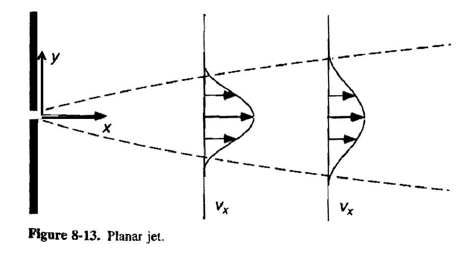
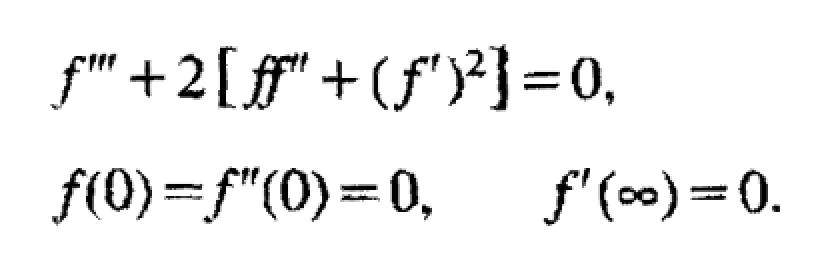
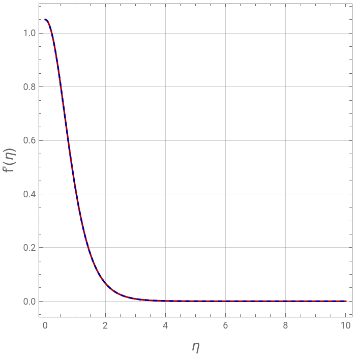
We compute the velocity profile created by a jet emerging from a narrow slit in a planar wall. The narrow jet of fluid is entering a large and stagnant volume of the same fluid. “An internal boundary layer is created by a narrow jet of fluid entering a large, stagnant volume of the same fluid. Some of the initial momentum of the jet is transferred to the outer fluid, causing it to be entrained. As this happens the jet gradually slows and spreads out” (extract from Deen’s textbook page 360)Hermann Schlichting (Boundary-Layer Theory, sixth edition. McGraw-Hill, New York, 1968, pp. 170-174) derived the governing equation (a split boundary value problem): Our numerical result obtained, using NDSolve and the shooting method , is compared to its counterpart obtained using an analytical expression derived in Deen’s textbook (Analysis of Transport Phenomena, William M. Deen, OUP, 1998). Values of parameters K and b are also computed. Finally, 3D, density and contour plots of the velocity distribution are presented.
We compute the velocity profile created by a jet emerging from a narrow slit in a planar wall. The narrow jet of fluid is entering a large and stagnant volume of the same fluid. “An internal boundary layer is created by a narrow jet of fluid entering a large, stagnant volume of the same fluid. Some of the initial momentum of the jet is transferred to the outer fluid, causing it to be entrained. As this happens the jet gradually slows and spreads out” (extract from Deen’s textbook page 360)Hermann Schlichting (Boundary-Layer Theory, sixth edition. McGraw-Hill, New York, 1968, pp. 170-174) derived the governing equation (a split boundary value problem): Our numerical result obtained, using NDSolve and the shooting method , is compared to its counterpart obtained using an analytical expression derived in Deen’s textbook (Analysis of Transport Phenomena, William M. Deen, OUP, 1998). Values of parameters K and b are also computed. Finally, 3D, density and contour plots of the velocity distribution are presented.
Acknowledgement :The governing equations and analytical solution are taken from the textbook Analysis of Transport Phenomena, William M. Deen, Oxford University Press, 1998.
In[]:=
Off[General::"spell1"]
Numerical solution
In[]:=
sol[ξ_]:=NDSolve[{D[f[η],{η,3}]+2(f[η]D[f[η],{η,2}]+(D[f[η],{η,1}])^2)0,f[0]0,f'[0]ξ,f''[0]0},{f[η]},{η,0,10}]
In[]:=
DFEnd[ξ_?NumericQ]:=D[f[η]/.sol[ξ],{η,1}]/.η10
In[]:=
SOL1=FindRoot[DFEnd[ξ]0,{ξ,0.5}]

Out[]=
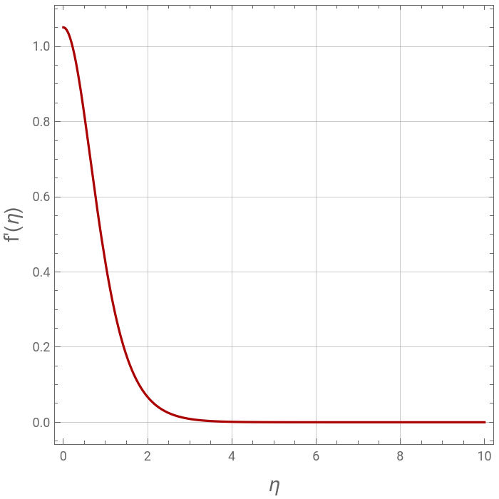
{ξ1.05094}
In[]:=
plt1=Plot[Evaluate[D[f[η]/.sol[ξ/.SOL1],{η,1}]],{η,0,10},PlotStyleDarker@Red,PlotRangeAll,FrameTrue,GridLinesAutomatic,AspectRatio1,ImageSize350{1,1},FrameLabel{Style["η",14],Style["f'(η)",14]}]
Out[]=
Determination of parameter b that appears in the analytical solution (in Deen's textbook) of the velocity
v
x
In[]:=
solt=Solve[b^2ξ/.SOL1,b]
Out[]=
{{b-1.02515},{b1.02515}}
Analytical solution
f'(η)=1-
2
b
2
(tanh(bη))
In[]:=
plt2=Plot(ξ/.SOL1)1-Tanh
ξ/.SOL1
η^2,{η,0,10},PlotStyle{Dashed,Darker@Blue},PlotRangeAll,FrameTrue,GridLinesAutomatic,AspectRatio1,ImageSize350{1,1},FrameLabel{Style["η",14],Style["f'(η)",14]}Out[]=
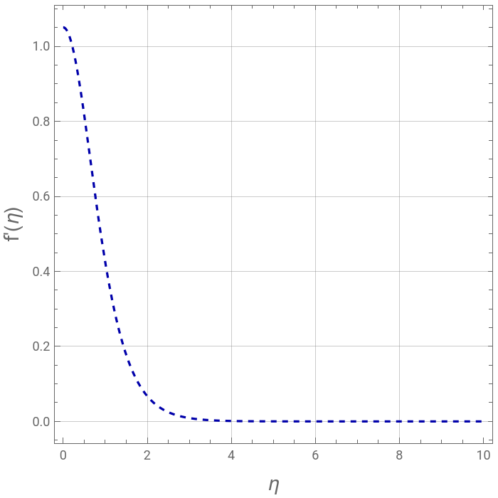
Comparing analytical and numerical solutions
In[]:=
Show[plt1,plt2]
Out[]=
Determination of parameter K that appears in the analytical solution (in Deen's textbook) of the velocity
v
x
CHECK: velocity normal to the wall @ x=8.69 and y=1.37
velocity normal to wall @ various distances from the wall (x=1, 2, 3, 4 and 5)