Consider the following experiment:
1. Start with a complete graph on n nodes—every node is connected to every other node.
2. Assign to each edge a random weight, chosen uniformly from the interval [0,1].
3. Compute the graph’s minimum spanning tree (MST).
4. Record the sum of the edge weights in that MST.
2. Assign to each edge a random weight, chosen uniformly from the interval [0,1].
3. Compute the graph’s minimum spanning tree (MST).
4. Record the sum of the edge weights in that MST.
Now repeat this process as grows larger and larger. The remarkable fact is this: the expected total weight of the random MST approaches the value of the Riemann zeta function at 3:
n
In[]:=
Style[[1]],12,FontFamily->"Arial"//Framed

Out[]=
In other words, a purely combinatorial-probabilistic process on random graphs unexpectedly leads you straight to the famous Apéry constant. This theorem was rigorously proved by A.M. Frieze based on the work of Walkup, P. Erdös and A. Rényi.
For visualization purpose, choose a small complete graph so that the labels are not too crowded:
In[]:=
n=7;
Uniformly assign the weight between [0,1] on each edge:
In[]:=
ew=RandomReal[{0,1},Binomial[n,2]];
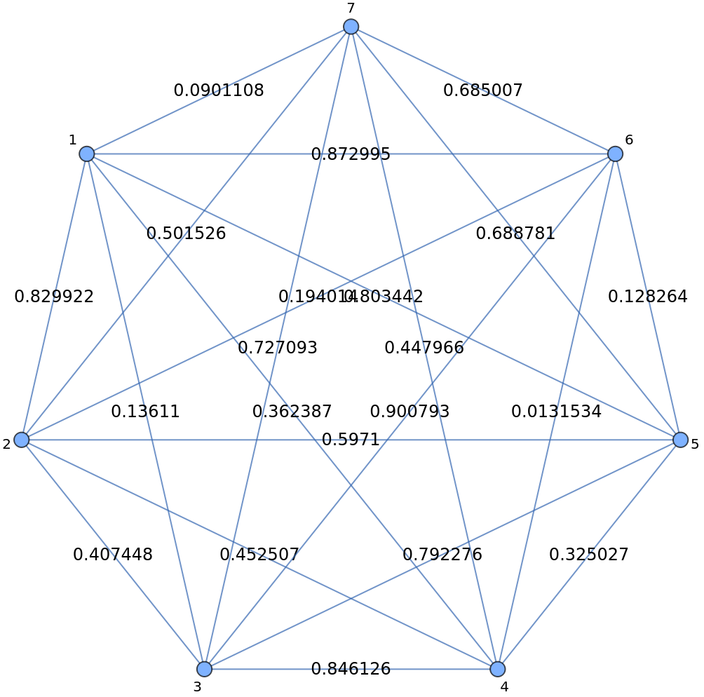
Visualize the graph with weight of edges:
In[]:=
g1=CompleteGraph[n,EdgeWeight->ew,EdgeLabels->"EdgeWeight",EdgeLabelStyle->12,VertexLabels->"Name"]
Out[]=
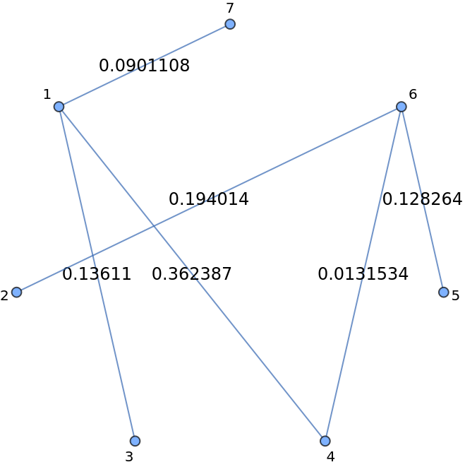
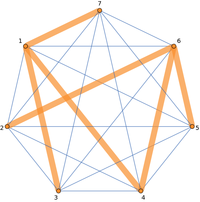
Find the minimum spanning tree as a subgraph with edge weights:
In[]:=
mst=FindSpanningTree[g1,VertexLabels->"Name"];Grid[{{mst,HighlightGraph[Annotate[g1,EdgeLabels->None],Style[mst,Thickness[0.03],StandardOrange]]}},Dividers->All]
Out[]=
Compute the length of the minimum spanning tree
In[]:=
AnnotationValue[mst,EdgeWeight]
Out[]=
{0.13611,0.362387,0.0901108,0.194014,0.0131534,0.128264}
In[]:=
Total[%]
Out[]=
0.924039
Do the same thing for of K-complete graphs for :
K=3,4,5,6,7,10,100,500
v={3,4,5,6,7,10,100,500};
In[]:=
res=Mean@Table[Total[AnnotationValue[FindSpanningTree@CompleteGraph[i,EdgeWeight->RandomReal[{0,1},Binomial[i,2]]],EdgeWeight]],{t,10},{i,v}]
Out[]=
{0.642456,0.860396,0.80748,1.08323,1.0249,1.00683,1.19652,1.21045,1.20355}
In[]:=
Grid[{v,res},Dividers->All]
Out[]=
3 | 4 | 5 | 6 | 7 | 10 | 100 | 500 | 1000 |
0.642456 | 0.860396 | 0.80748 | 1.08323 | 1.0249 | 1.00683 | 1.19652 | 1.21045 | 1.20355 |
We can also test the theorem repeatedly for large complete graph with parallel kernels:
In[]:=
LaunchKernels[];
Test on 1000 copies of 1000-complete graphs with random edge weights:
In[]:=
nv=1000;data=ParallelTable[Total[AnnotationValue[FindSpanningTree@CompleteGraph[nv,EdgeWeight->RandomReal[{0,1},Binomial[nv,2]]],EdgeWeight]],{i,1000}];
The distribution of the lengths of their minimum spanning trees:
In[]:=
Histogram[data,{0.005}]
Out[]=
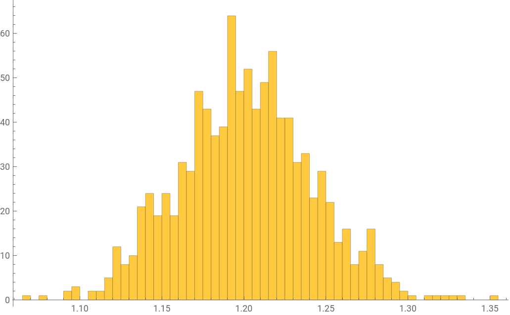
The value is close to ζ(3):
In[]:=
{Mean[data],Zeta[3.]}
Out[]=
{1.20125,1.20206}
Reference
Reference
A.M. Frieze, On the value of a random minimum spanning tree problem, Discrete Applied Mathematics, Volume 10, Issue 1, 1985,Pages 47-56, ISSN 0166-218X, https://doi.org/10.1016/0166-218X(85)90058-7.
CITE THIS NOTEBOOK
CITE THIS NOTEBOOK
Random minimum spanning trees and Riemann Zeta function
by Shenghui Yang
Wolfram Community, STAFF PICKS, November 17, 2025
https://community.wolfram.com/groups/-/m/t/3577126
by Shenghui Yang
Wolfram Community, STAFF PICKS, November 17, 2025
https://community.wolfram.com/groups/-/m/t/3577126