ABSTRACT (original article): Viruses play a crucial role in regulating prokaryotic populations, yet their impact on subsurface environments, specifically groundwater habitats, remains poorly understood. In this study, we employed the virus-dilution approach to measure lytic virus production rates in shallow groundwater located near the city of Vienna (Austria) during the period from July−November 2020. Physico-chemical parameters (pH, electrical conductivity, water temperature, concentration of dissolved oxygen), prokaryotic, and viral abundance, and viral decay rates were monitored as well. Our findings revealed low virus-to-prokaryote ratios varying between 0.9−3.9 throughout the study period and a lack of correlation between prokaryotic and viral abundance in groundwater. Virus production rates varied between 9−12% of viral abundance in July−August and between 34−36% of viral abundance in October−November. Seasonal variations in virus production rates were found to be correlated with electrical conductivity, revealing ~3.5 times higher virus production rates during periods with high electrical conductivity and low groundwater recharge in October−November compared to July−August with higher groundwater recharge and lower electrical conductivity. Our data indicate that groundwater recharge disrupts the balance between virus and prokaryotic host communities, resulting in a deficiency of suitable prokaryotic host cells for viral proliferation. CITATION (original article): Pleyer D, Griebler C, Winter C (2024), Virus production in shallow groundwater at the bank of the Danube River. PLoS ONE 19(8): e0306346. https://doi.org/10.1371/journal.pone.0306346
-1
h
-1
h
The notebook contains the calculations used to statistically explore a small data set on virus production and viral decay in shallow groundwater near the Danube River. Surprisingly, virus production was well correlated with electrical conductivity within groundwater suggesting that groundwater recharge appears to be a driving force for virus production at the sampling station.
Virus production (VP) in groundwater
Virus production (VP) in groundwater
VP already corrected for abundance differences between in situ and in vitro, Auxiliary Data
Data
Data
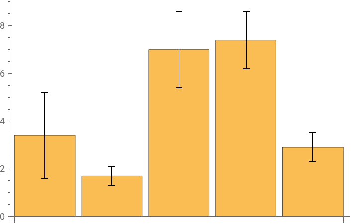
Virus production data (vpground only for groundwater).
vp={Around[3.4,1.8],Around[1.7,0.4],Around[7.0,1.6],Around[7.4,1.2],Around[2.9,0.6]};vpground={Around[3.4,1.8],Around[1.7,0.4],Around[7.0,1.6],Around[7.4,1.2]};
Virus production data for each individual experiment (vpdetailground only for groundwater).
vpdetail={{4.8,4.0,1.3},{2.1,1.4,1.7},{8.7,7.0,5.4},{6.2,8.7},{3.6,2.3}};vpdetailground={{4.8,4.0,1.3},{2.1,1.4,1.7},{8.7,7.0,5.4},{6.2,8.7}};
Sampling dates.
date={DateList["30 Jul 2020"],DateList["25 Aug 2020"],DateList["08 Oct 2020"],DateList["25 Nov 2020"],DateList["25 Nov 2020"]};
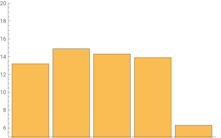
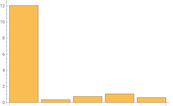
Auxiliary data (...ground only for groundwater): temperature (°C), concentration of oxygen (mg L^-1), pH, electrical conductivity (µSi cm^-1), prokaryotic abundance (Nx10^4 mL^-1), viral abundance (Nx10^4 mL^-1), virus-to-prokaryotes ratio.
temp={13.2,14.9,14.3,13.9,6.3};tempground={13.2,14.9,14.3,13.9};oxygen={0.63,1.08,0.76,0.36,12.05};oxygenground={0.63,1.08,0.76,0.36};ph={7.52,"n.d.",7.13,7.24,8.10};phground={7.52,"n.d.",7.13,7.24};cond={513,495,573,590,424};condground={513,495,573,590};prok={9.4,16.7,13.9,15.5,44.3};prokground={9.4,16.7,13.9,15.5};vir={36.2,14.5,19.7,22.0,596.2};virground={36.2,14.5,19.7,22.0};vpr=vir/prok;vprground=Drop[vpr,-1];
Spearman Rank Correlations
Spearman Rank Correlations
Data Graphics
Data Graphics
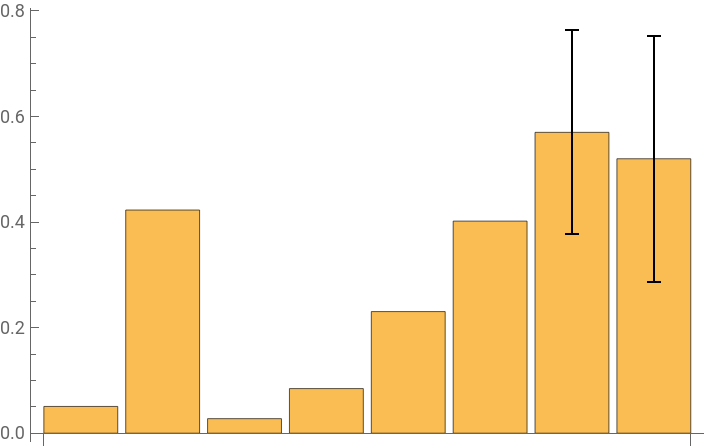
Coefficient of variation.
In[]:=
BarChart[{StandardDeviation[tempground]/Mean[tempground],StandardDeviation[oxygenground]/Mean[oxygenground],StandardDeviation[Delete[phground,2]]/Mean[Delete[phground,2]],StandardDeviation[condground]/Mean[condground]//N,StandardDeviation[prokground]/Mean[prokground],StandardDeviation[virground]/Mean[virground],StandardDeviation[vpground]/Mean[vpground],StandardDeviation[ficground]/Mean[ficground]}]
Out[]=
In[]:=
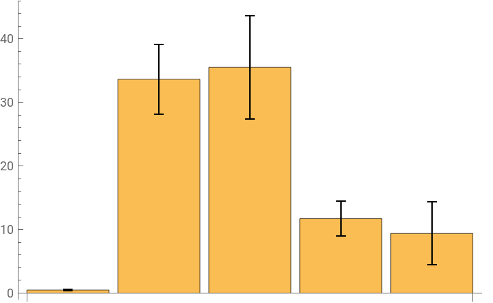
BarChart[Reverse[(vp/vir)*100]]
Out[]=
In[]:=
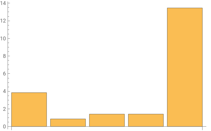
BarChart[vpr]
Out[]=
In[]:=
BarChart[vp]
Out[]=
In[]:=
BarChart[temp,PlotRange->{5,20}]
Out[]=
In[]:=
BarChart[Reverse[oxygen]]
Out[]=
In[]:=
BarChart[ph,PlotRange->{7,8.5}]
In[]:=
BarChart[Reverse[cond],PlotRange->{400,600}]
In[]:=
BarChart[Reverse[vir]]
In[]:=
BarChart[prok]
Precipitation and Water Level of Danube river
Precipitation and Water Level of Danube river
Sampling dates expressed as number of rows within datasets (precipitation.csv and level.csv).
In[]:=
sampling={30,56,100,148};
Import precipitation data from file "precipitation.csv"; precipitation in mm.
In[]:=
precipitation=Transpose[Drop[Transpose[Import["/Users/cwinter/Documents/Vienna/Daniel/PloSONE/NiederschlagsWasserstandDaten/precipitation.csv"]],1]];
Vertical lines mark months of the year .
Conductivity plot based on sampling dates as overlay for precplot and levelplot .
Import water level data from file "level.csv"; water level in m at station Korneuburg.
Virus Decay
Virus Decay
Import data
Calculate decay models and produce virus decay graphs from data for each sampling event (kritz1-4).
CITE THIS NOTEBOOK
CITE THIS NOTEBOOK
Virus production in shallow groundwater at the bank of the Danube River
by Daniel Pleyer, Christian Griebler, Christian Winter
Wolfram Community, STAFF PICKS, October 2, 2024
https://community.wolfram.com/groups/-/m/t/3289943
by Daniel Pleyer, Christian Griebler, Christian Winter
Wolfram Community, STAFF PICKS, October 2, 2024
https://community.wolfram.com/groups/-/m/t/3289943