Introduction
Introduction
Linear Programming is arguably one of the most ‘obviously’ useful areas of mathematics, as you will see in a minute. It is interesting, then, that it is not generally seen until degree level, particularly when the skills it needs are very low-level - any keen fourteen year-old would be able to understand it, and implement it (certainly for the example we will consider). For that reason I won’t present you with any prerequisites, and we will dive right in: I will say that this will be a very brief ‘computational lecture’, as the Wolfram Language (as it is for many things) is powerful in regard to it, so most of our time will be spent looking at the theory behind what is going on.
Linear Programming - what is it?
Linear Programming - what is it?
Linear Programming is defined as the ‘optimisation’ of an ‘objective function’ according to ‘linear constraints’. We will explore each of those terms in a different order, so they make more sense.
The ‘objective function’ takes in several variables that represent their real-life counterparts. For example, x may be the number of analogue watches a factory makes, y the number of digital watches. The objective function deals with these variables depending on what we want to optimise, for example the time of production, profit, or cost of manufacturing. In this way we may set our objective function to be P = 30x+20y, if P is the profit in pounds, and analogue watches give a profit of £30, and digital watches £20. We will return to this example later, so keep it in mind!
‘Linear constraints’ are inequalities which limit our variables. It could be the case that there are not enough materials to make more than 300 watches, in which case x+y ≤ 300. Because it is linear programming we will only be dealing with linear inequalities - that is to say, the powers of x and y will only ever be 1. It’s worth noting that this is often the way it is in real-life, so we won’t look into ways we could deal with more complicated constraints.
Finally, ‘optimisation’ is the process of minimising or maximising our objective function, using those constraints mentioned above. It is hopefully obvious, now, that without our constraints optimisation would generally set x and y to negative or positive infinity, depending on the objective function and whether we were maximising or minimising it. As always, all this should appear clearer with a proper example.
Visualising Linear Programming Problems
Visualising Linear Programming Problems
Let’s return to our watch problem. We are going to present it as such:
Maximise P = 30x + 20y, subject to:
x ≥ 2y
3x + 5y ≤ 200
x+2y ≤ 100
x, y ≥ 0
Where x and y are the number of analogue and digital watches respectively.
The above is a generally accepted form of problem, although you may see it written differently at higher levels. It is worth noting that our first constraint, x ≥ 2y, means that there need to be at least two analogue watches for every digital watch. In real life this may be because they’re more popular. The next two constraints may deal with certain materials, some of which are needed more for digital watches, but of which there are limited amounts. The last constraint means that we cannot produce a negative amount of either watch (obviously this is a must in real life, so we generally see this in all problems).
The astute reader may realise that, for a two-variable problem like this, we can represent it on a graph. Let’s do so.
‘RegionPlot[]’ takes in inequalities, separated by &&, and bound within the limits given at the end.
In[]:=
RegionPlot[x≥2y&&3x+5y≤200&&x+2y≤100,{x,0,100},{y,0,40}]
Out[]=
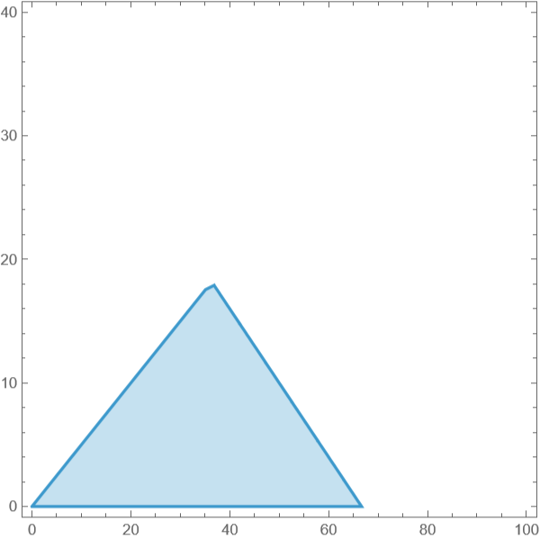
As you can see, we get a helpful visualisation showing us only the area we need to worry about. The lines for each inequality are essentially ‘cut off’, so you may wish to imagine them proceeding. Generally, we would draw them out entirely and then shade in the area we need. All points within this area satisfy the constraints given.
Most of the time there is an ‘optimal point’ that allows us to achieve the maximum or minimum value of the objective function. We can find this point in several ways, but I would like to leave it to you to explore those methods, for we have an easier option available to us.
Most of the time there is an ‘optimal point’ that allows us to achieve the maximum or minimum value of the objective function. We can find this point in several ways, but I would like to leave it to you to explore those methods, for we have an easier option available to us.
The LinearOptimization Function
The LinearOptimization Function
This function is the holy grail in regard to Linear Programming. Before we use it, we must note one thing - it can only be used to minimise a function. At first thought this seems problematic for our above watch-profit. But we can circumvent this problem with ease and a little bit of intuition. Let’s negate our objective function, so it becomes -P = -30x - 20y. If we minimise it and then find x and y as we would usually, that same x and y will actually give us the maximum value of our profit function. The most negative value, in other words, is by definition the greatest positive value if we negate it once again. Therefore we run Wolfram’s function as follows:
This function takes arguments in the order Objective Function, Constraints, and Result Constraints, where the latter detail (in this case) that x and y must be integers, as we cannot make part of a watch (logically speaking).
In[]:=
LinearOptimization[-30x-20y,{x≥2y,3x+5y≤200,x+2y≤100,x≥0,y≥0},{x∈Integers,y∈Integers}]
Out[]=
{x66,y0}
It is, quite frankly, as simple as that. To maximise our Profit we should therefore make 66 analogue watches and no digital watches. Of course, this wouldn’t be the case in industry - we would have far more constraints, because some people certainly still prefer digital watches. But in this case we would expect a profit of 30*66 or £1980.
It is worth realising the great simplicity of what we have looked at. It is also worth realising that it is easily expandable. Where computational solving is very useful is when we see three or more variables, because the former is hard to visualise, and the latter impossible to visualise. It also becomes increasing complicated to solve it by hand. But that, more or less, is that.
It is worth realising the great simplicity of what we have looked at. It is also worth realising that it is easily expandable. Where computational solving is very useful is when we see three or more variables, because the former is hard to visualise, and the latter impossible to visualise. It also becomes increasing complicated to solve it by hand. But that, more or less, is that.
Conclusion
Conclusion
I said that this would be brief, and I hope that I haven’t disappointed you in that respect. I have purposefully left a few gaps here and there (such as in regard to manual computation) for you to look at, as it remains simple but is the sort of thing that is best to practice yourself. I would highly recommend reading the documentation for this function:
https://reference.wolfram.com/language/ref/LinearOptimization.html
It is very useful indeed, and has a few nice examples (and visualisations, too) which should lead on well from here. I myself think that it’s a shame this topic isn’t covered at lower levels of education, given its simplicity and real-world applications. All the same, I thank you for reading this, and hope that it has served as a good introduction to linear programming for those who have never encountered it before, especially within the Wolfram Language. Until the next time!