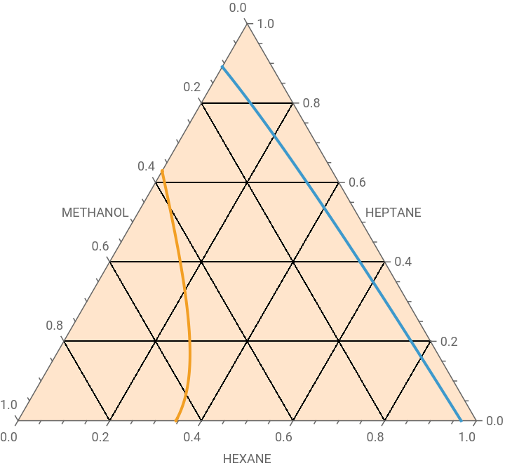
The liquid-liquid equilibrium (LLE) behavior of the methanol–heptane–hexane ternary system at 32.85 °C was investigated using the NRTL activity coefficient model. The common tangent plane (CTP) equations were first solved to obtain an initial equilibrium point, and an arc-length continuation procedure was subsequently employed to trace the entire two-phase boundary. This approach successfully generated the Type II LLE diagram and provided a continuous representation of the equilibrium branches without repeatedly solving independent phase equilibrium calculations.
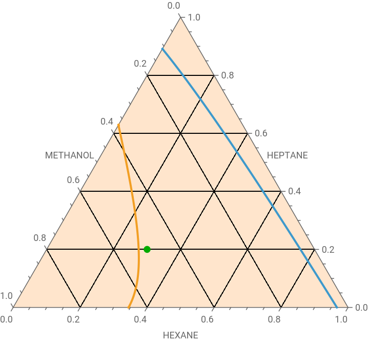
The thermodynamic stability of the feed composition (z={0.30,0.20,0.50}) was then evaluated using the tangent plane distance (TPD) criterion. The global minimization produced (TPD_{min}=-0.00453334), indicating that the feed composition is thermodynamically unstable and will undergo liquid-liquid phase separation. The composition of the incipient phase was found to be (w*={0.56865,0.38065,0.05071}), confirming that the selected feed lies inside the miscibility gap.
The equilibrium tie line associated with this unstable feed was subsequently determined using two independent procedures. First, a classical liquid-liquid equilibrium calculation based on equality of component activities and overall mass balances was solved using FindRoot. Second, the same tie line was directly extracted from the CTP arc-length continuation solution. Both methods yielded identical equilibrium compositions, namely (x_alpha={0.28143,0.18736,0.53121}) and (x_beta={0.56622,0.38121,0.05257}), demonstrating excellent agreement and validating the continuation-based methodology.
A second feed composition, (z={0.10,0.10,0.80}), was also analyzed to verify the stability criterion outside the two-phase region. In this case, the TPD minimization yielded (TPD_{min}=3.44*10^-15), which is essentially zero, and the minimizing composition coincided with the feed composition itself. Therefore, the mixture is thermodynamically stable and remains as a single liquid phase. These results demonstrate that the combined CTP, arc-length continuation, and TPD framework provides a reliable and efficient methodology for identifying stable and unstable regions, determining tie lines, and characterizing complex ternary liquid-liquid equilibrium behavior.
LLE diagram using the method based on common tangent plane and arc-length continuation
NRTL Parameters -- Source: Aspen-Plus v .14
ClearAll["Global`*"];
Universal gas constant
R=1.9872041;
Temperature
T=273.15+32.85;
NRTL Parameters
a13=0.42399900;a12=0.301800;a32=0.440800;t31=1287.78000;t13=1915.07700;t23=1598.3120000;t32=1566.43700;t12=-285.9411;t21=252.997600;α={{0.,a12,a13},{a12,0.,a32},{a13,a32,0.}};τ={{0.,t12,t13},{t21,0.,t23},{t31,t32,0.}}/(RT);
NRTL tau_{ij} matrix (dimensionless, at T ≈ 298 K
τ//TableFormα//TableForm
Out[]//TableForm=
0. | -0.470233 | 3.14936 |
0.416057 | 0. | 2.62844 |
2.11777 | 2.57602 | 0. |
Out[]//TableForm=
0. | 0.3018 | 0.423999 |
0.3018 | 0. | 0.4408 |
0.423999 | 0.4408 | 0. |
G[i_,j_]:=Exp[-α[[i,j]]τ[[i,j]]];
Composition vector
xvec[x1_,x2_]:={x1,x2,1-x1-x2};
NRTL Activity coefficients
lnGamma[i_,x1_,x2_]:=Module[{x,term1,term2},x=xvec[x1,x2];term1=Sum[x[[j]]τ[[j,i]]G[j,i],{j,1,3}]/Sum[x[[k]]G[k,i],{k,1,3}];term2=Sum[x[[j]]G[i,j]/Sum[x[[k]]G[k,j],{k,1,3}](τ[[i,j]]-Sum[x[[m]]τ[[m,j]]G[m,j],{m,1,3}]/Sum[x[[m]]G[m,j],{m,1,3}]),{j,1,3}];term1+term2];gamma[i_,x1_,x2_]:=Exp[lnGamma[i,x1,x2]];
Dimensionless Gibbs energy of mixing : g/RT
gmix[x1_,x2_]:=Module[{x},x=xvec[x1,x2];Sum[x[[i]]Log[x[[i]]],{i,1,3}]+Sum[x[[i]]lnGamma[i,x1,x2],{i,1,3}]];
Derivatives
dgdx1[x1_,x2_]:=Evaluate[D[gmix[u,v],u]/.{u->x1,v->x2}];dgdx2[x1_,x2_]:=Evaluate[D[gmix[u,v],v]/.{u->x1,v->x2}];
Unknowns
vars={x1a,x2a,x1b,x2b,m1,m2};
Common tangent equations
eq1=dgdx1[x1a,x2a]-m1==0;eq2=dgdx1[x1b,x2b]-m1==0;eq3=dgdx2[x1a,x2a]-m2==0;eq4=dgdx2[x1b,x2b]-m2==0;eq5=gmix[x1b,x2b]-gmix[x1a,x2a]==(m1(x1b-x1a)+m2(x2b-x2a));
Extra constraint - Prevent trivial solution xα=xβ
In[]:=
eq6=(x1b-x1a)^2+(x2b-x2a)^2==d;
a small d=0.07 yield an initial point
In[]:=
d0t=0.07;
Solution
solct=FindRoot[{eq1,eq2,eq3,eq4,eq5,eq6/.d->d0t},{{x1a,0.33},{x2a,0.4},{x1b,0.060},{x2b,0.4},{m1,-0.65},{m2,-0.45}},MaxIterations->1000]
Out[]=
{x1a0.0100149,x2a0.882978,x1b0.00706729,x2b0.618419,m1-4.54248,m20.0315688}
In[]:=
init={x1a[0]==(x1a/.solct),x2a[0]==(x2a/.solct),x1b[0]==(x1b/.solct),x2b[0]==(x2b/.solct),m1[0]==(m1/.solct),m2[0]==(m2/.solct),d[0]==d0t}
Out[]=
{x1a[0]0.0100149,x2a[0]0.882978,x1b[0]0.00706729,x2b[0]0.618419,m1[0]-4.54248,m2[0]0.0315688,d[0]0.07}
In[]:=
initdev={x1a'[0]==0.01,x2a'[0]==0.01,x1b'[0]==0.01,x2b'[0]==0.01,m1'[0]==0.01,m2'[0]==0.01,d'[0]==0.01}
Out[]=
{[0]0.01,[0]0.01,[0]0.01,[0]0.01,[0]0.01,[0]0.01,[0]0.01}
′
x1a
′
x2a
′
x1b
′
x2b
′
m1
′
m2
′
d
In[]:=
SYS={eq1,eq2,eq3,eq4,eq5,eq6}/.x1a->x1a[s]/.x1b->x1b[s]/.x2a->x2a[s]/.x2b->x2b[s]/.m1->m1[s]/.m2->m2[s]/.d->d[s];
In[]:=
auxeq=x1a'[s]^2+x1b'[s]^2+x2a'[s]^2+x2b'[s]^2+m1'[s]^2+m2'[s]^2+d'[s]^2==1
Out[]=
2
′
d
2
′
m1
2
′
m2
2
′
x1a
2
′
x1b
2
′
x2a
2
′
x2b
In[]:=
SYSFinal=Join[SYS,{auxeq},init,initdev];
In[]:=
SOL=Quiet@NDSolve[SYSFinal,{x1a,x2a,x1b,x2b,m1,m2,d},{s,-100,100},AccuracyGoal->5]
Out[]=
x1aInterpolatingFunction,x2aInterpolatingFunction,x1bInterpolatingFunction,x2bInterpolatingFunction,m1InterpolatingFunction,m2InterpolatingFunction,dInterpolatingFunction


In[]:=
DATA1=Table[{x1a[s],x2a[s],1-x1a[s]-x2a[s]}/.SOL,{s,-7.85,16.0,0.01}];DATA2=Table[{x1b[s],x2b[s],1-x1b[s]-x2b[s]}/.SOL,{s,-7.85,16.0,0.01}];
In[]:=
Pt={{2,1},{0,Sqrt[3.]}}/2;
Type II liquid-liquid equilibrium (LLE) diagram
In[]:=
p0=Show[TernaryListPlot[{Flatten[DATA1,1],Flatten[DATA2,1]},Joined->True,PlotStyle->Thick,GridLines->Automatic,FrameLabel->{"HEXANE","HEPTANE","METHANOL"},PlotRange->All,Method->{"Backdrop"->LightOrange}]]
Out[]=
Feed composition
z={0.30,0.20,0.50};
In[]:=
Show[p0,Graphics[{Darker@Green,PointSize[0.02],Point[Pt.{z[[1]],z[[2]]}]}]]
Out[]=
NRTL Activity coefficients
In[]:=
gammaNRTL[x_List]:=Module[{n=3,lngamma,s1,s2,s3},lngamma=Table[0.,{n}];Do[s1=Sum[x[[j]]*τ[[j,i]]*G[j,i],{j,1,n}];s2=Sum[x[[j]]*G[j,i],{j,1,n}];s3=Sum[(x[[j]]*G[i,j]/Sum[x[[k]]*G[k,j],{k,1,n}])*(τ[[i,j]]-Sum[x[[m]]*τ[[m,j]]*G[m,j],{m,1,n}]/Sum[x[[m]]*G[m,j],{m,1,n}]),{j,1,n}];lngamma[[i]]=s1/s2+s3;,{i,1,n}];Exp[lngamma]];
TPD Function
Global minimum of TPD
Results
Fetch tie line that goes through z = {0.3, 0.2, 0.5} classical method based on FindRoot
Fetch tie line that goes through z = {0.3, 0.2, 0.5} new method based on our CTP and arc-length continuation
Let us draw this particular tie line in dashed cyan
Let us consider another feed z ={0.1,0.8,0.1}. This time we expect minimum of TPD to be positive
TPD Function
Global minimum of TPD
Results
CITE THIS NOTEBOOK
CITE THIS NOTEBOOK
CTP, arc-length continuation, and TPD analysis for methanol-heptane-hexane system
by Housam Binous
Wolfram Community, STAFF PICKS, June 16, 2026
https://community.wolfram.com/groups/-/m/t/3734453
by Housam Binous
Wolfram Community, STAFF PICKS, June 16, 2026
https://community.wolfram.com/groups/-/m/t/3734453