This study compares two image restoration approaches — TSVD and Autoencoder — applied to low-resolution natural images from the BSD100 dataset. SVD is first introduced to reveal the low-rank structure of images — a few dominant singular values carry most of the visual information while the small ones carry mostly noise — which motivates the use of its truncated variant, TSVD. Since both the original high-resolution and low-resolution versions are available, the high-resolution images serve as ground truth for quantitative evaluation. Each method is evaluated using PSNR and SSIM metrics to determine which approach most effectively restores image quality. By comparing a classical linear algebra approach and a deep learning approach under the same controlled conditions, this research aims to provide practical insight into which method works best for general image restoration tasks.
Why Does Image quality Matter?
Why Does Image quality Matter?
The Problem with Low-Resolution Images
The Problem with Low-Resolution Images
Where Low-Quality Images Appear in Real Life
Where Low-Quality Images Appear in Real Life
Low-quality images are more common than we might think. Security cameras, inexpensive sensors, and budget smartphones all produce images that lack the resolution to clearly identify important details. To see what this low resolution looks like, we will load a real example from the BSD100 dataset. This dataset is the most widely used benchmark collection in image restoration research.
Load a high-resolution BSD100 image and its 4× downsampled version, and display them side by side:
In[]:=
dataDir=NotebookDirectory[];hrDir=FileNameJoin[{dataDir,"BSD100_HR"}];lrDir=FileNameJoin[{dataDir,"BSD100_LR_x4"}];imgHR=Import[FileNameJoin[{hrDir,"3096.png"}]];imgLR=Import[FileNameJoin[{lrDir,"3096.png"}]];GraphicsGrid[{{imgHR,imgLR}},Frame->All,PlotLabel->{"High Resolution (Original)","Low Resolution (Input)"}]
Out[]=
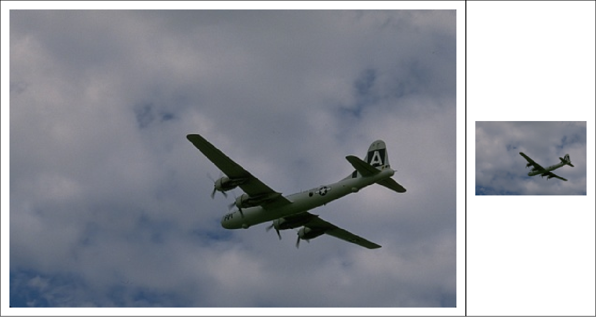
The image on the left is the original high-resolution version. The image on the right is the low-resolution version. The image on the right is what we are trying to restore. Even from this simple comparison, we can see clearly that the meaningful visual information has been lost.
Why Existing Solutions Are Hard to Use
Why Existing Solutions Are Hard to Use
Most existing research focuses on complex algorithms that require high computing power, making them difficult to apply in practice. This study approaches by comparing two methods: one is rooted in classical linear algebra and the other is based on deep learning. To find out which one works best in an accessible and interpretable way is the conclusion we are trying to reach.
What We’re Trying to Do
What We’re Trying to Do
Research Question
Research Question
This study asks a simple question: When TSVD and Autoencoder are applied to the same dataset under the same conditions, which one produces the best results?
Compare the pixel dimensions of the HR and LR images:
In[]:=
{ImageDimensions[imgHR],ImageDimensions[imgLR]}
Out[]=
{{481,321},{120,80}}
The output confirms that the LR image is approximately a quarter of the size of the HR image in both width and height. This means that the resolution was reduced by a factor of 4.
What We Expect to Find
What We Expect to Find
TSVD is expected to perform reliably due to their mathematical stability, while the Autoencoder is expected to handle complex image patterns more flexibly. However, whether the added complexity of a deep learning model always leads to better results is exactly what this study hopes to clarify.
Two Different Ways to Restore an Image
Two Different Ways to Restore an Image
The Math Approach — SVD and TSVD
The Math Approach — SVD and TSVD
What Is SVD?
What Is SVD?
When we look at a digital image, it is essentially a matrix which is a grid of numbers where each number represents the brightness of a pixel. SVD(Singular Value Decomposition) is a technique that breaks this matrix down into three components: U, S, and V (Andrews & Patterson, 1976). What makes this useful is that S contains a ranked list of values that tell us how important each piece of information is. The first few values are large and capture the overall structure of the image. The rest are small and correspond to fine details or noise.
Plot the LR image’s singular values in descending order:
mat=ImageData[imgLR][[All,All,1]];{u,s,v}=SingularValueDecomposition[mat];ListPlotDiagonal[s],
Out[]=
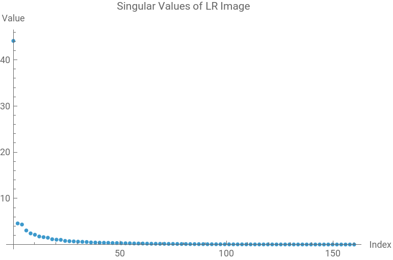
The plot shows a sharp drop after the first few singular values. The first value is close to 44.1, but by the 10th value it has already fallen to 2.1, and after that the values remain nearly flat and close to zero all the way to index 160. This tells us that the vast majority of the visual information in this image is concentrated in just the first few pieces. In other words, we do not need all 160 singular values to reconstruct a recognizable image.
This is the key idea behind TSVD which keeps only the most significant pieces and discarding the rest.
This is the key idea behind TSVD which keeps only the most significant pieces and discarding the rest.
Reconstructing an Image from Its Top Components
Reconstructing an Image from Its Top Components
The plot above shows that only a few singular values are large, and this is true for almost any natural image. The SVD lets us rebuild an image by stacking up simple pieces, one for each singular value, starting with the most important:
A = σ₁u₁v₁ᵀ + σ₂u₂v₂ᵀ + ... + σₙuₙvₙᵀ
How much each pieces uᵢvᵢᵀ matters depends on its singular value σᵢ. The first few pieces have a large σ and capture the main shapes and colors of the image. The later pieces have a small σ and only add fine detail — and the very last ones are mostly noise.
This suggests a simple idea: keep only the first k pieces and drop the rest. The result still holds the important structure but leaves out the noisy tail. This is called a rank-k approximation, and keeping the top-k pieces is provably the best you can do with that few (Eckart & Young, 1936) — the smaller the pieces we throw away, the less we lose.
Of course, this only works if the small singular values really are just noise, and not some hidden detail we actually need. So before trusting truncation, let’s test that assumption directly.
A = σ₁u₁v₁ᵀ + σ₂u₂v₂ᵀ + ... + σₙuₙvₙᵀ
How much each pieces uᵢvᵢᵀ matters depends on its singular value σᵢ. The first few pieces have a large σ and capture the main shapes and colors of the image. The later pieces have a small σ and only add fine detail — and the very last ones are mostly noise.
This suggests a simple idea: keep only the first k pieces and drop the rest. The result still holds the important structure but leaves out the noisy tail. This is called a rank-k approximation, and keeping the top-k pieces is provably the best you can do with that few (Eckart & Young, 1936) — the smaller the pieces we throw away, the less we lose.
Of course, this only works if the small singular values really are just noise, and not some hidden detail we actually need. So before trusting truncation, let’s test that assumption directly.
Reconstruct the image weighting each component by 1/σᵢ, amplifying the smallest singular values to test whether they hold real signal:
In[]:=
mat=ImageData[imgLR][[All,All,1]];{u,s,v}=SingularValueDecomposition[mat];nSingular=Min[Dimensions[s]];sFullInv=DiagonalMatrix[Table[1/s[[i,i]],{i,nSingular}]];restored=u.sFullInv.Transpose[v[[All,1;;nSingular]]];imgRestoredPinv=Image[Clip[restored,{0,1}]];{imgLR,imgRestoredPinv}
Out[]=
,
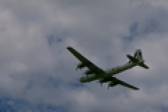
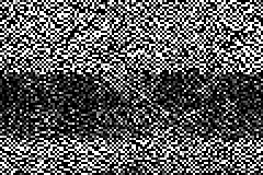
Here we try the opposite of truncation on purpose. Normally each piece is weighted by its singular value σᵢ. This time we weight it by 1/σᵢ instead, which gives the largest weight to the smallest pieces — the very ones we suspect are just noise. If those small pieces really did hold useful structure, the rebuilt image would still look like the original. Instead, it turns into pure noise.
The reason is simple. A singular value as small as σᵢ = 0.001 turns into a weight of 1/σᵢ = 1000. So even a tiny bit of noise in that piece gets multiplied a thousand times and drowns out the whole image.
This confirms what we suspected: the small singular values carry almost no real signal. Just noise that blows up when we give it weight. So the right move is not to amplify these pieces but to throw them away. Keeping only the top-k pieces does exactly that.
The reason is simple. A singular value as small as σᵢ = 0.001 turns into a weight of 1/σᵢ = 1000. So even a tiny bit of noise in that piece gets multiplied a thousand times and drowns out the whole image.
This confirms what we suspected: the small singular values carry almost no real signal. Just noise that blows up when we give it weight. So the right move is not to amplify these pieces but to throw them away. Keeping only the top-k pieces does exactly that.
What Is TSVD and Why Is It Different?
What Is TSVD and Why Is It Different?
Instead of reconstructing the image from all singular values, TSVD (Truncated SVD) keeps only the top k pieces and discards the rest (Eckart & Young, 1936). The largest values hold the main structure of the image, so keeping just a few already reproduces most of what we see, while the small tail— the noise-dominated pieces we just saw — contributes very little. The choice of k is a trade-off: too few and the image stays blurry, enough and the structure comes back sharply.
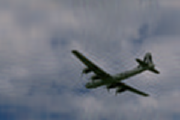
Reconstruct the image with TSVD at k = 5, 10, 20, 30 to watch detail return as k grows:
In[]:=
Table[Module[{channels,restoredChannels,result},channels=ColorSeparate[imgLR];restoredChannels=Table[Module[{mat,u,s,v,restored},mat=ImageData[channels[[c]]];{u,s,v}=SingularValueDecomposition[mat];restored=u[[All,1;;k]].s[[1;;k,1;;k]].Transpose[v[[All,1;;k]]];Image[restored]],{c,3}];result=ColorCombine[restoredChannels];Labeled[ImageResize[result,300],"k = "<>ToString[k]]],{k,{5,10,20,30}}]
Out[]=
,
,
,
k = 5 |

k = 10 |

k = 20 |
k = 30 |
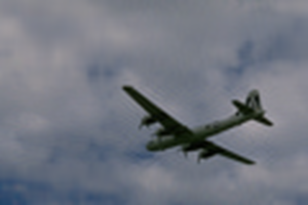
At k=5, the overall structure of the scene is visible, but the image looks blurry with noticeable color artifacts. At k=10, the quality improves dramatically. The artifact has gone and the outline of the airplane starts to come up, but still the background is blurry. At k=20, the shapes become sharp, most of the color distortion disappears, and airplane and the cloud is distinguished. Compared to k=10 the improvement is noticeable. At k=30, the improvement over k=20 is relatively small.
This suggests that the most critical visual information is captured between k=20 and k=30, and beyond k=30 adding more singular values brings diminishing returns. Therefore, k=20 was selected as the optimal value for the subsequent. The choice of k is known to significantly affect restoration quality (Sanborn, 2019). That is something we will measure precisely using PSNR and SSIM in a later section.
This suggests that the most critical visual information is captured between k=20 and k=30, and beyond k=30 adding more singular values brings diminishing returns. Therefore, k=20 was selected as the optimal value for the subsequent. The choice of k is known to significantly affect restoration quality (Sanborn, 2019). That is something we will measure precisely using PSNR and SSIM in a later section.
The AI Approach — Autoencoder
The AI Approach — Autoencoder
How an Autoencoder Works
How an Autoencoder Works
While SVD and TSVD rely on mathematical structure, an Autoencoder takes a completely different approach. It is a neural network that learns from data (Mao et al., 2016). During training, it is shown thousands of image pairs and learns to map degraded inputs to clean outputs. The network first compresses the image into a compact internal representation, then reconstructs it with the missing details filled in. No mathematical formula is written by hand since the network figures it out on its own.
Why We Use a Pretrained Model
Why We Use a Pretrained Model
Training an Autoencoder from scratch requires large amounts of data and significant computing time, which is beyond the scope of this study. Instead, we use a pretrained model from the Wolfram Neural Net Repository called VDSR(Very Deep Net for Super-Resolution). It was trained on 291 images and is designed specifically for recovering a high-resolution image from a low-resolution input (Kim et al., 2016).
Apply the pretrained VDSR network to the LR image and compare input, result, and HR original:
The three images show the LR input, the Autoencoder result, and the HR original side by side. Compared to the LR input, the Autoencoder result shows noticeably sharper edges and clearer details. Without any explicit mathematical formula, the pretrained network was able to recover a visually convincing result. However, whether this improvement is actually better than what SVD and TSVD achieved is a question we will answer precisely in the next chapter using PSNR and SSIM.
How We Measure Success
How We Measure Success
PSNR
PSNR
To compare the three methods objectively, we need a consistent way to measure restoration quality. PSNR(Peak Signal-to-Noise Ratio) compares the restored image to the original pixel by pixel and expresses the difference in decibels (Banham & Katsaggelos, 1997). A higher PSNR means the restored image is closer to the original.
Compute the PSNR of the TSVD reconstruction (k=20) against the HR original:
This gives us a PSNR of 32.54 dB for TSVD at k=20. One detail is worth making explicit: the truncation operates on the low-resolution image at its native size (120×80), and the increase to high-resolution dimensions is done separately by interpolation (ImageResize). The TSVD step therefore acts as a low-rank approximation of the LR image, not as the upscaling itself — the resize is what changes the dimensions.
We will apply the same calculation to TSVD and Autoencoder results in the next chapter to make a direct comparison.
We will apply the same calculation to TSVD and Autoencoder results in the next chapter to make a direct comparison.
SSIM
SSIM
PSNR measures numerical accuracy, but it does not always reflect how the image actually looks to a human observer. Two images can have the same PSNR but look very different to the eye. This is where SSIM comes in. SSIM(Structural Similarity Index Measure) evaluates brightness, contrast, and structure together, mimicking the way human vision perceives image quality (Wang et al., 2004). A score of 1 means the restored image is identical to the original, and a score closer to 0 means it looks very different.
Compute the SSIM of the same TSVD reconstruction:
The result is 0.976, which is very close to 1. This suggests that the TSVD-restored image at k=20 is structurally very similar to the original. Together with the PSNR of 32.54 dB, these numbers illustrate how the two metrics behave on a single image. This particular image is mostly smooth sky, which is unusually easy to approximate with a low rank, so its scores are higher than average. The real baseline for our comparison will be the average PSNR and SSIM across 30 images, which we compute in the next chapter.
Comparing the Three Methods
Comparing the Three Methods
SVD and TSVD — Measuring Performance Across 30 Images
SVD and TSVD — Measuring Performance Across 30 Images
In an earlier section, we applied each method to a single image and observed the results visually. However, a single image is not enough to draw reliable conclusions. To get a more objective picture, we now apply TSVD and the Autoencoder to 30 randomly selected images from the BSD100 test set and calculate the average PSNR and SSIM across all of them.
Select 30 random BSD100 images as the evaluation set (seeded for reproducibility):
Compute the average TSVD (k=20) PSNR across all 30 test images:
Define an SSIM helper and compute the average TSVD SSIM across the 30 images:
The average PSNR for TSVD at k=20 is 22.79 dB and the average SSIM is 0.913. These two numbers will serve as the baseline for comparison with the Autoencoder.
Autoencoder — How Does AI Compare?
Autoencoder — How Does AI Compare?
We now apply the same evaluation to the Autoencoder across the same 30 test images.
Compute the Autoencoder’s average PSNR across the same 30 images:
Compute the Autoencoder’s average SSIM across the same 30 images:
Comparing these numbers, the two methods show a split result. TSVD at k=20 achieves a higher PSNR (22.79 dB vs 22.17 dB), while the Autoencoder scores higher on SSIM (0.918 vs 0.913). This mixed outcome suggests that neither method is strictly superior. Each captures a different aspect of image quality.
Side-by-Side Comparison
Side-by-Side Comparison
To make the comparison as clear as possible, let’s visualize all the results in a single chart.
Chart the average PSNR of both methods side by side:
Chart the average SSIM of both methods side by side:
The two charts reveal a nuanced result. In terms of PSNR, TSVD at k=20 achieves an average of 22.79 dB compared to 22.17 dB for the Autoencoder, meaning the mathematical approach reconstructs pixel values more accurately. However, in terms of SSIM, the result is reversed: the Autoencoder scores 0.918 compared to 0.913 for TSVD.
This outcome is interesting because the two metrics measure different things. PSNR measures how close the pixel values are to the original, while SSIM measures how similar the image looks to human vision. At first glance, TSVD does better on pixel accuracy, and the Autoencoder does slightly better on perceptual structure.
This outcome is interesting because the two metrics measure different things. PSNR measures how close the pixel values are to the original, while SSIM measures how similar the image looks to human vision. At first glance, TSVD does better on pixel accuracy, and the Autoencoder does slightly better on perceptual structure.
Are the Differences Statistically Significant?
Are the Differences Statistically Significant?
The averages above point to a split result, but the gaps are small — 0.62 dB and 0.005. Before reading too much into them, we should check whether they are real or just a result of which 30 images we happened to pick. Since every image is restored by both methods, we can compare them image by image: for each image we take the difference between the two scores and ask whether the average difference is really different from zero. We use a paired t-test for this, and we also run the Wilcoxon signed-rank test as a backup, because it does not assume the data is normally distributed.
For PSNR, TSVD scores 0.62 dB higher than the Autoencoder on average. Both tests confirm that this gap is significant (paired t-test p ≈ 5 × 10⁻¹¹; Wilcoxon p ≈ 2 × 10⁻⁶). The gap is small, but it appears in almost every image, so the paired test detects it clearly. This means TSVD’s higher pixel accuracy is real, not just a result of the particular images we sampled.
For SSIM, the result is less clear. The Autoencoder scores 0.005 higher on average, and the paired t-test gives p ≈ 0.039, which looks significant. But the test also warns that the SSIM differences are not normally distributed (p ≈ 8 × 10⁻⁶), so the t-test is not reliable here. The Wilcoxon test, which does not need this assumption, gives p ≈ 0.11 — above the 0.05 threshold. Following the more reliable test, the SSIM difference is not significant. In other words, the Autoencoder’s small SSIM lead may just be noise.
Putting both results together gives a clearer picture than the averages alone. TSVD is significantly better on PSNR, while on SSIM the two methods are statistically the same.
For SSIM, the result is less clear. The Autoencoder scores 0.005 higher on average, and the paired t-test gives p ≈ 0.039, which looks significant. But the test also warns that the SSIM differences are not normally distributed (p ≈ 8 × 10⁻⁶), so the t-test is not reliable here. The Wilcoxon test, which does not need this assumption, gives p ≈ 0.11 — above the 0.05 threshold. Following the more reliable test, the SSIM difference is not significant. In other words, the Autoencoder’s small SSIM lead may just be noise.
Putting both results together gives a clearer picture than the averages alone. TSVD is significantly better on PSNR, while on SSIM the two methods are statistically the same.
What Does This Tell Us?
What Does This Tell Us?
Math vs AI — Key Takeaways
Math vs AI — Key Takeaways
The results give a clear but careful conclusion. Across 30 BSD100 images, the two methods are much closer than people usually assume. Many expect deep learning to be clearly better, but that is not what we found. When the two methods do differ, TSVD is the one with the advantage. TSVD scored higher on PSNR (22.79 dB vs 22.17 dB), and the paired test shows this difference is real. The Autoencoder scored a little higher on SSIM (0.918 vs 0.913), but this difference was not significant when we used the more reliable test. So we can say that TSVD is clearly better at pixel accuracy, and the two methods are equal in perceptual quality.
This result is different from the common idea that a deep learning model is always better than a classical math method. In this study, a simple and low-cost method (TSVD) performed as well as a pretrained deep network. It was even better on one metric (PSNR), and the two methods were equal on the other (SSIM). However, this result applies only to our setup: one pretrained model, a 4× downsampling task, and a simple global SSIM. So it does not prove that classical methods are as good as every deep learning model. What it shows is that the difference between classical and AI methods is smaller than many people expect, and that small differences in scores should be checked with a statistical test before we accept them.
In the end, the better method depends on the goal. If pixel accuracy is most important, TSVD is the better choice, because its advantage is reliable. If perceptual quality is most important, the two methods are basically equal, so other points decide the question: TSVD is simpler, faster, and easier to understand. The study does not show that one method is always better. It shows that a classical method is still a strong and practical option next to a modern deep model.
This result is different from the common idea that a deep learning model is always better than a classical math method. In this study, a simple and low-cost method (TSVD) performed as well as a pretrained deep network. It was even better on one metric (PSNR), and the two methods were equal on the other (SSIM). However, this result applies only to our setup: one pretrained model, a 4× downsampling task, and a simple global SSIM. So it does not prove that classical methods are as good as every deep learning model. What it shows is that the difference between classical and AI methods is smaller than many people expect, and that small differences in scores should be checked with a statistical test before we accept them.
In the end, the better method depends on the goal. If pixel accuracy is most important, TSVD is the better choice, because its advantage is reliable. If perceptual quality is most important, the two methods are basically equal, so other points decide the question: TSVD is simpler, faster, and easier to understand. The study does not show that one method is always better. It shows that a classical method is still a strong and practical option next to a modern deep model.
Limitations and Future Direction
Limitations and Future Direction
What This Study Could Not Cover
What This Study Could Not Cover
There are several limitations worth acknowledging. First, this study used only one pretrained Autoencoder model(VDSR), which may not represent the full potential of deep learning for this task.
Second, TSVD was evaluated at k=20, selected based on a visual comparison across k=5, 10, 20, and 30 on a single image. A more rigorous quantitative search across all 100 images could further validate this choice and potentially identify a better k.
Third, we evaluated the methods on 30 images from BSD100. A paired test on this sample showed that the PSNR difference is significant, but the SSIM difference is not. Because the SSIM gap is very small, 30 images may not be enough to detect it. A larger sample would help us see whether the two methods are truly equal on SSIM, or whether the difference is just too small to find here.
Second, TSVD was evaluated at k=20, selected based on a visual comparison across k=5, 10, 20, and 30 on a single image. A more rigorous quantitative search across all 100 images could further validate this choice and potentially identify a better k.
Third, we evaluated the methods on 30 images from BSD100. A paired test on this sample showed that the PSNR difference is significant, but the SSIM difference is not. Because the SSIM gap is very small, 30 images may not be enough to detect it. A larger sample would help us see whether the two methods are truly equal on SSIM, or whether the difference is just too small to find here.
What Could Be Done Next
What Could Be Done Next
Several directions could extend this work. Training a custom Autoencoder directly on BSD100 rather than using a pretrained model would provide a fairer comparison (Bigdeli & Zwicker, 2017). Testing across a wider range of k values with quantitative evaluation across all 100 images would better justify the choice of k. Extending the evaluation to other standard benchmark datasets such as Set5 or Set14 would also help determine whether the results generalize beyond BSD100. Finally, incorporating a more sophisticated patch-based SSIM implementation would produce more reliable quality assessments.
References
References
◼
Eckart, C., & Young, G. (1936). The approximation of one matrix by another of lower rank. Psychometrika, 1(3), 211–218.
◼
Andrews, H. C., & Patterson, C. L. (1976). Singular Value Decompositions and Digital Image Processing, 24(1), 26–53.
◼
Banham, M. R., & Katsaggelos, A. K. (1997). Digital Image Restoration.
◼
Wang, Z., Bovik, A. C., Sheikh, H. R., & Simoncelli, E. P. (2004). Image Quality Assessment: From Error Visibility to Structural Similarity. IEEE Transactions on Image Processing, 13(4), 600–612.
◼
Mao, X.-J., Shen, C., & Yang, Y.-B. (2016). Image Restoration Using Convolutional Auto-encoders with Symmetric Skip Connections. arXiv:1606.08921
◼
Kim, J., Lee, J. K., & Lee, K. M. (2016). Accurate Image Super-Resolution Using Very Deep Convolutional Networks. Proceedings of the IEEE Conference on Computer Vision and Pattern Recognition (CVPR), 1646–1654.
◼
Bigdeli, S. A., & Zwicker, M. (2017). Image Restoration Using Autoencoding Priors. arXiv:1703.09964.
AI Assistance
AI Assistance
This content was developed with AI assistance from Claude (Anthropic), used as a coding assistant for debugging Wolfram Language syntax and implementing the PSNR/SSIM and statistical comparison code. The AI drew on no external sources; all references are my own. I reviewed, ran, and tested all code, understood every part of the work, and made the research and interpretation decisions myself.
CITE THIS NOTEBOOK
CITE THIS NOTEBOOK
TSVD and autoencoder for image restoration: a comparative study
by Jaekyung Seol
Wolfram Community, STAFF PICKS, June 3, 2026
https://community.wolfram.com/groups/-/m/t/3726674
by Jaekyung Seol
Wolfram Community, STAFF PICKS, June 3, 2026
https://community.wolfram.com/groups/-/m/t/3726674