In Ref. 1, the influence of several parameters for a continuous evaporation (temperature, absolute pressure, feed flow, dry matter of feed solution) of an alcoholic extract was investigated using Doehlert matrices. Here, we reproduces some of the main results for model determination. In addition, statistical and ANOVA analyses are provided.
coded values of the four factors
In[]:=
Doehlert[nFac_,ncenter_]:=Module[{RegularSimplex,iFac},RegularSimplex=Table[0,{i,1,nFac(nFac+1)+ncenter},{j,1,nFac}];For[i=1,i<=nFac,i++,For[j=1,j<=i,j++,{If[i==j,RegularSimplex[[i+1,j]]=Sqrt[i+1]/Sqrt[2i],RegularSimplex[[i+1,i-j]]=1/Sqrt[2(i-(j-1))(i-j)]]}]]iFac=0;For[i=1,i<=nFac+1,i++,For[j=2,j<=nFac+1,j++,{If[i≠j,{iFac=iFac+1,RegularSimplex[[nFac+1+iFac]]=RegularSimplex[[i]]-RegularSimplex[[j]]}]}]];Table[RegularSimplex[[i,j]]//N,{i,1,nFac(nFac+1)+ncenter},{j,1,nFac}]]
In[]:=
nFac=4;ncenter=1;
In[]:=
M=Doehlert[nFac,ncenter];
In[]:=
M//TableForm
Out[]//TableForm=
0. | 0. | 0. | 0. |
1. | 0. | 0. | 0. |
0.5 | 0.866025 | 0. | 0. |
0.5 | 0.288675 | 0.816497 | 0. |
0.5 | 0.288675 | 0.204124 | 0.790569 |
-1. | 0. | 0. | 0. |
-0.5 | -0.866025 | 0. | 0. |
-0.5 | -0.288675 | -0.816497 | 0. |
-0.5 | -0.288675 | -0.204124 | -0.790569 |
0.5 | -0.866025 | 0. | 0. |
0.5 | -0.288675 | -0.816497 | 0. |
0.5 | -0.288675 | -0.204124 | -0.790569 |
-0.5 | 0.866025 | 0. | 0. |
0. | 0.57735 | -0.816497 | 0. |
0. | 0.57735 | -0.204124 | -0.790569 |
-0.5 | 0.288675 | 0.816497 | 0. |
0. | -0.57735 | 0.816497 | 0. |
0. | 0. | 0.612372 | -0.790569 |
-0.5 | 0.288675 | 0.204124 | 0.790569 |
0. | -0.57735 | 0.204124 | 0.790569 |
0. | 0. | -0.612372 | 0.790569 |
In[]:=
Dimensions[%]
Out[]=
{21,4}
Range for factors (Pressure in hPa, Volume flow in l/hr, Temperature in °C, Weight fraction in %) are used to map coded to real values
In[]:=
low={121,5.27,36.6,-0.23};high={179,8.73,73.4,3.77};mid={150,7.0,55,1.77};
In[]:=
0.5(low+high)
Out[]=
{150.,7.,55.,1.77}
In[]:=
halfrange=0.5(high-low)
Out[]=
{29.,1.73,18.4,2.}
In[]:=
realvar=Table[mid[[j]]+M[[i,j]]halfrange[[j]],{i,1,21},{j,1,4}];
In[]:=
realvar//TableForm
Out[]//TableForm=
150. | 7. | 55. | 1.77 |
179. | 7. | 55. | 1.77 |
164.5 | 8.49822 | 55. | 1.77 |
164.5 | 7.49941 | 70.0235 | 1.77 |
164.5 | 7.49941 | 58.7559 | 3.35114 |
121. | 7. | 55. | 1.77 |
135.5 | 5.50178 | 55. | 1.77 |
135.5 | 6.50059 | 39.9765 | 1.77 |
135.5 | 6.50059 | 51.2441 | 0.188861 |
164.5 | 5.50178 | 55. | 1.77 |
164.5 | 6.50059 | 39.9765 | 1.77 |
164.5 | 6.50059 | 51.2441 | 0.188861 |
135.5 | 8.49822 | 55. | 1.77 |
150. | 7.99882 | 39.9765 | 1.77 |
150. | 7.99882 | 51.2441 | 0.188861 |
135.5 | 7.49941 | 70.0235 | 1.77 |
150. | 6.00118 | 70.0235 | 1.77 |
150. | 7. | 66.2677 | 0.188861 |
135.5 | 7.49941 | 58.7559 | 3.35114 |
150. | 6.00118 | 58.7559 | 3.35114 |
150. | 7. | 43.7323 | 3.35114 |
Forming MD the Computation Matrix
In[]:=
x1=Transpose[M][[1]]
Out[]=
{0.,1.,0.5,0.5,0.5,-1.,-0.5,-0.5,-0.5,0.5,0.5,0.5,-0.5,0.,0.,-0.5,0.,0.,-0.5,0.,0.}
In[]:=
x2=Transpose[M][[2]]
Out[]=
{0.,0.,0.866025,0.288675,0.288675,0.,-0.866025,-0.288675,-0.288675,-0.866025,-0.288675,-0.288675,0.866025,0.57735,0.57735,0.288675,-0.57735,0.,0.288675,-0.57735,0.}
In[]:=
x3=Transpose[M][[3]]
Out[]=
{0.,0.,0.,0.816497,0.204124,0.,0.,-0.816497,-0.204124,0.,-0.816497,-0.204124,0.,-0.816497,-0.204124,0.816497,0.816497,0.612372,0.204124,0.204124,-0.612372}
In[]:=
x4=Transpose[M][[4]]
Out[]=
{0.,0.,0.,0.,0.790569,0.,0.,0.,-0.790569,0.,0.,-0.790569,0.,0.,-0.790569,0.,0.,-0.790569,0.790569,0.790569,0.790569}
In[]:=
x1x1
Out[]=
{0.,1.,0.25,0.25,0.25,1.,0.25,0.25,0.25,0.25,0.25,0.25,0.25,0.,0.,0.25,0.,0.,0.25,0.,0.}
In[]:=
x2x2
Out[]=
{0.,0.,0.75,0.0833333,0.0833333,0.,0.75,0.0833333,0.0833333,0.75,0.0833333,0.0833333,0.75,0.333333,0.333333,0.0833333,0.333333,0.,0.0833333,0.333333,0.}
In[]:=
x3x3
Out[]=
{0.,0.,0.,0.666667,0.0416667,0.,0.,0.666667,0.0416667,0.,0.666667,0.0416667,0.,0.666667,0.0416667,0.666667,0.666667,0.375,0.0416667,0.0416667,0.375}
In[]:=
x4x4
Out[]=
{0.,0.,0.,0.,0.625,0.,0.,0.,0.625,0.,0.,0.625,0.,0.,0.625,0.,0.,0.625,0.625,0.625,0.625}
In[]:=
x1x2
Out[]=
{0.,0.,0.433013,0.144338,0.144338,0.,0.433013,0.144338,0.144338,-0.433013,-0.144338,-0.144338,-0.433013,0.,0.,-0.144338,0.,0.,-0.144338,0.,0.}
In[]:=
x1x3
Out[]=
{0.,0.,0.,0.408248,0.102062,0.,0.,0.408248,0.102062,0.,-0.408248,-0.102062,0.,0.,0.,-0.408248,0.,0.,-0.102062,0.,0.}
In[]:=
x1x4
Out[]=
{0.,0.,0.,0.,0.395285,0.,0.,0.,0.395285,0.,0.,-0.395285,0.,0.,0.,0.,0.,0.,-0.395285,0.,0.}
In[]:=
x2x3
Out[]=
{0.,0.,0.,0.235702,0.0589256,0.,0.,0.235702,0.0589256,0.,0.235702,0.0589256,0.,-0.471405,-0.117851,0.235702,-0.471405,0.,0.0589256,-0.117851,0.}
In[]:=
x2x4
Out[]=
{0.,0.,0.,0.,0.228218,0.,0.,0.,0.228218,0.,0.,0.228218,0.,0.,-0.456435,0.,0.,0.,0.228218,-0.456435,0.}
In[]:=
x3x4
Out[]=
{0.,0.,0.,0.,0.161374,0.,0.,0.,0.161374,0.,0.,0.161374,0.,0.,0.161374,0.,0.,-0.484123,0.161374,0.161374,-0.484123}
In[]:=
MD=Transpose[{{1.0000,1.0000,1.0000,1.0000,1.0000,1.0000,1.0000,1.0000,1.0000,1.0000,1.0000,1.0000,1.0000,1.0000,1.0000,1.0000,1.0000,1.0000,1.0000,1.0000,1.0000},x1,x2,x3,x4,x1x1,x2x2,x3x3,x4x4,x1x2,x1x3,x1x4,x2x3,x2x4,x3x4}];
In[]:=
Grid[Table[NumberForm[MD[[i,j]],{4,4}],{i,1,21},{j,1,15}],Frame->All]
Out[]=
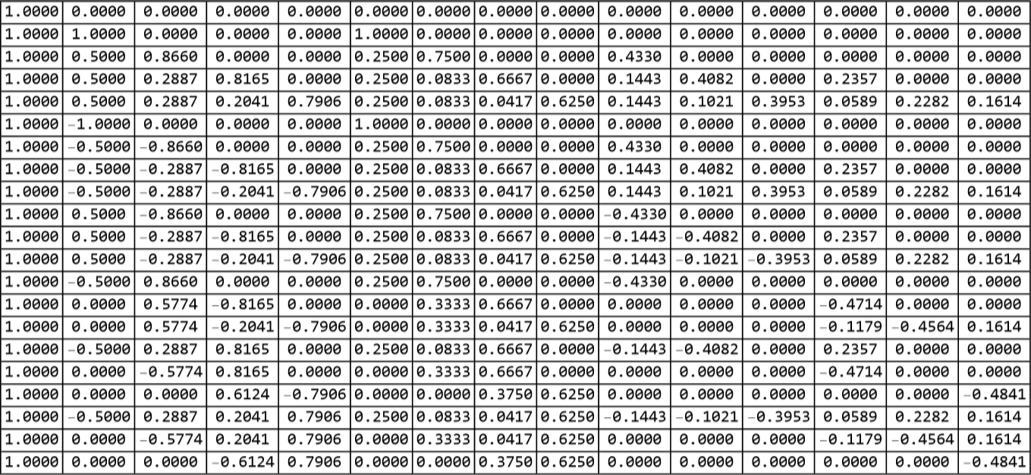
Response Productivity (in kg/hr) is labelled y
In[]:=
y={0.1049,0.1047,0.1249,0.1129,0.2132,0.1032,0.0825,0.0958,0.0102,0.0828,0.097,0.0924,0.1253,0.1215,0.0129,0.1151,0.0883,0.0116,0.2087,0.1607,0.198};
In[]:=
y//TableForm
Out[]//TableForm=
0.1049 |
0.1047 |
0.1249 |
0.1129 |
0.2132 |
0.1032 |
0.0825 |
0.0958 |
0.0102 |
0.0828 |
0.097 |
0.0924 |
0.1253 |
0.1215 |
0.0129 |
0.1151 |
0.0883 |
0.0116 |
0.2087 |
0.1607 |
0.198 |
Determination of the quadratic model by multilinear regression of the continuous evaporation process
Determination of the quadratic model by multilinear regression of the continuous evaporation process
Model determination using LinearModelFit of Mathematica
We take advantage of Mathematica’s capabilities in order to provide a thorough statistical analysis.
A small p-value (typically < 0.05) means the variable significantly contributes to explaining the outcome.
A large p-value suggests the variable may not be important in the model and should be dropped from the model equation.
Response’s vector is labelled y
Dry matter (%)
Dry matter (%)
Determination of the quadratic model by multilinear regression of the continuous evaporation process
Determination of the quadratic model by multilinear regression of the continuous evaporation process
Model determination using LinearModelFit of Mathematica
We take advantage of Mathematica’s capabilities in order to provide a thorough statistical analysis.
A small p-value (typically < 0.05) means the variable significantly contributes to explaining the outcome.
A large p-value suggests the variable may not be important in the model and should be dropped from the model equation.
We take advantage of Mathematica’s capabilities in order to provide a thorough statistical analysis.
A small p-value (typically < 0.05) means the variable significantly contributes to explaining the outcome.
A large p-value suggests the variable may not be important in the model and should be dropped from the model equation.
References
References
◼
[1] H. Fauduet, C. Porte, J.-L. Havet and David Daguet, Modelling of influential parameters on a continuous evaporation process by Doehlert shells, Journal of Automated Methods & Management in Chemistry, Vol. 25, No. 1 (2003) pp. 21–30.
◼
We also used the ideas for Placing a ContourPlot under a Plot3D from: https://community.wolfram.com/groups/-/m/t/1148582
CITE THIS NOTEBOOK
CITE THIS NOTEBOOK
Doehlert matrix for the optimization of continuous evaporation process
by Housam Binous and Ahmed Bellagi
Wolfram Community, STAFF PICKS, November 1, 2025
https://community.wolfram.com/groups/-/m/t/3569104
by Housam Binous and Ahmed Bellagi
Wolfram Community, STAFF PICKS, November 1, 2025
https://community.wolfram.com/groups/-/m/t/3569104