Thermodynamic Modeling of Ternary LLE (pyridine–water–chlorobenzene at 25°C and 1 atm)
Housam Binous and Abdelmalek Hasseine
Housam Binous and Abdelmalek Hasseine
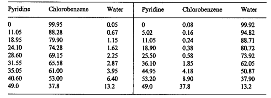
This notebook presents a complete thermodynamic modeling for the ternary liquid-liquid equilibrium (LLE) system pyridine–water–chlorobenzene at 25°C and 1 atm. It takes the experimental tie-line data (in weight fractions), fits an NRTL (Non-Random Two-Liquid) activity coefficient model to that data, and then uses the fitted parameters to reconstruct the full binodal curve and tie-line network on a ternary diagram.Part A The code begins by hard-coding the raw experimental LLE data (extract and raffinate weight fractions of pyridine, water, and chlorobenzene) into a table, then converts everything to mole fractions using each component’s molecular weight.A block of nested Module definitions implements the NRTL equations themselves: the binary interaction parameters, the τ (tau) and G parameters derived from those interaction energies, and finally the activity coefficient expression for each component in a multicomponent mixture. This is the standard three-suffix NRTL formulation extended to three components, with the non-randomness parameter α typically fixed (0.2) and the energy parameters left as the adjustable unknowns.The “hybrid method” (using hybrid PSO + interior-point approach) combines two fitting strategies at once: matching activity/equilibrium relationships (isoactivity conditions between extract and raffinate phases and minimizing deviation from the experimental phase-split . The code assembles a sum-of-squared-residuals objective function comparing model-predicted phase compositions against the experimental tie-line data. It then calls a global optimizer (PSO) as a first pass, refined by a local/interior-point method using FindMinimum in order to search for the NRTL binary interaction parameters that best reproduce all nine experimental tie lines simultaneously.Part B Once the NRTL parameters are fixed, Part B shifts to generating the entire phase diagram rather than just the nine known points. It defines the molar Gibbs energy of mixing (via the NRTL activity coefficients) as a function over the ternary composition space, then constructs the common tangent plane condition — the thermodynamic requirement that two coexisting liquid phases share the same tangent plane to the Gibbs energy surface. This is the rigorous way to locate binodal (phase boundary) points rather than relying on interpolation between experimental tie lines.Solving the common-tangent-plane equations directly is numerically delicate near the plait point, where the two phases merge and the system becomes ill-conditioned. The “arc-length continuation” method handles this by parameterizing solutions along the arc length of the phase boundary curve rather than by composition directly, allowing the solver to step smoothly around the nose of the binodal curve and through the plait point without the Jacobian becoming singular.The final portion of the code takes the computed binodal points and tie lines and renders them using Mathematica’s ternary plotting utilities (TernaryListPlot or a custom triangular coordinate transform), overlaying the calculated phase boundary, the reconstructed tie lines, and the plait point onto the triangular diagram — visually reproducing (and extending) the classic pyridine/water/chlorobenzene phase diagram from Treybal, but generated entirely from the fitted NRTL model rather than raw experimental interpolation.Together, the two parts form a self-contained thermodynamic modeling exercise: Part A answers “what NRTL parameters best describe this system?” and Part B answers “what does the complete phase diagram look like according to that model?” — including regions between and beyond the original nine experimental tie lines, which is valuable for extraction process design where you need equilibrium data at compositions the original experiments didn’t directly measure.References:[1] Peake, J. S.; Thompson, K. E., Jr. “Four Ternary Liquid Systems Involving Monochlorobenzene: Phase Equilibria and Tie Line Data.” Industrial and Engineering Chemistry 1952, 44 (10), 2439–2441. https://pubs.acs.org/doi/10.1021/ie50514a044[2] Treybal, R. E. Mass-Transfer Operations, 3rd ed. New York: McGraw-Hill Book Company, 1980.
Part A: NRTL model determination using Hybrid method
Part A: NRTL model determination using Hybrid method
Determination of NRTL parameters is based on a Hybrid PSO - InteriorPoint approach
LLE data from Refs. 1-2 in wt %
In[]:=
(*convertwt\b%intomol%usingmolecularweightsof79.10(pyridine),18.02(water),and112.56g/mol(chlorobenzene)*)(*ExtractPhase:{Pyridine,Water,Chlorobenzene}inmole%*)extractPhase={{0.000,0.312,99.688},{14.534,3.869,81.597},{23.644,6.300,70.056},{28.893,8.528,62.580},{32.846,11.346,55.808},{34.963,13.965,51.072},{36.794,18.206,45.000},{38.321,26.524,35.155},{36.698,43.407,19.894}};(*RaffinatePhase:{Pyridine,Water,Chlorobenzene}inmole%*)raffinatePhase={{0.000,99.987,0.013},{1.191,98.782,0.027},{2.758,97.200,0.042},{5.059,94.870,0.071},{7.276,92.608,0.116},{11.651,87.930,0.420},{16.572,82.345,1.083},{23.554,73.677,2.769},{36.698,43.407,19.894}};
In[]:=
ClearAll[NC,T,NTIL,xxexp,yyexp,P,z];T=298.15;data=Table[Join[extractPhase[[i]]/100,raffinatePhase[[i]]/100],{i,1,Length@raffinatePhase}];
{m,n}=Dimensions[data];NC=n/2;NTIL=m;x1e=data[[All,1]];x2e=data[[All,2]];x3e=data[[All,3]];x1r=data[[All,4]];x2r=data[[All,5]];x3r=data[[All,6]];(*PHASERAFFINATE/PHASEEXTRACTforpyridine(1)+water(2)+chlorobenzene(3)ternarysystem*)xxexp={x1r,x2r,x3r};yyexp={x1e,x2e,x3e};
In[]:=
NRTL[x_]:=Module[{R=1.987,alp,tau,G,gam,G1,tau1,G2,s,act,aa,bb,zz,i,j},alp=Table[0.,{NC},{NC}];alp[[1,2]]=0.2;alp[[1,3]]=0.2;alp[[2,3]]=0.2;alp[[2,1]]=alp[[1,2]];alp[[3,1]]=alp[[1,3]];alp[[3,2]]=alp[[2,3]];tau=Table[P[[i,j]]/T,{i,NC},{j,NC}];G=Table[Exp[-alp[[i,j]]tau[[i,j]]],{i,NC},{j,NC}];gam=Table[0.,{NC}];G1=Table[0.,{NC},{NC}];tau1=Table[0.,{NC},{NC}];G2=Table[0.,{NC},{NC}];s=Table[0.,{NC},{NC}];Do[aa=0.;bb=0.;Do[zz=G[[j,i]]x[[j]];aa+=zz;bb+=zztau[[j,i]];,{j,NC}];gam[[i]]=bb/aa;Do[G1[[j,i]]=G[[j,i]]/aa;tau1[[j,i]]=tau[[j,i]]-gam[[i]];G2[[j,i]]=G1[[j,i]]tau1[[j,i]];s[[j,i]]=x[[i]]G2[[j,i]];,{j,NC}];,{i,NC}];Do[Do[gam[[i]]+=s[[i,j]],{j,NC}];gam[[i]]=Exp[gam[[i]]];,{i,NC}];act=Table[x[[i]]gam[[i]],{i,NC}];act]
In[]:=
EQUILIBRE[X_]:=Module[{x,y,act1,act2,f,Xt,Yt,i},x=Take[X,NC];y=Take[X,{NC+1,2NC}];act1=NRTL[x];act2=NRTL[y];f=Table[0.,{2NC+1}];Do[f[[i]]=act1[[i]]-act2[[i]],{i,NC}];Xt=Sum[X[[i]],{i,NC}];Yt=Sum[X[[i]],{i,NC+1,2NC}];f[[NC+1]]=1-Xt;f[[NC+2]]=1-Yt;Do[f[[NC+2+i]]=z[[i]]-X[[i]]X[[2NC+1]]-X[[i+NC]](1-X[[2NC+1]]),{i,NC-1}];f]
Part B: LLE diagram computation using common tangent plane and arc - length continuation
Part B: LLE diagram computation using common tangent plane and arc - length continuation
Method based on common tangent plane and arc - length continuation
NRTL Model Parameters at T=298.15 K from my above hybrid optimization code and stored in P
tau_ij for pyridine (1) + water (2) + chlorobenzene (3)
Alpha matrix (symmetric)
Composition vector
NRTL activity coefficients
Dimensionless Gibbs energy of mixing: g/RT
Derivatives
Unknowns
Common tangent equations
Extra constraint - Prevent trivial solution xα=xβ
First value for d --- very small d=0.0001 yield approximately the plait point
First value for d --- very small d=0.0001 yield approximately the plait point
Solution is near {0.367,0.434}
Type I liquid-liquid equilibrium (LLE) diagram - Plait point indicated in red
water-rich phase {x1,x2,x3}, CB-rich phase {x1,x2,x3}
Display as tables with headers
Combine into tie-line pairs:{phaseI,phaseII}
Show all nine experimental tie lines
Let us compute the RMSD