ABSTRACT (original article): This paper introduces a framework for finite non-cooperative games where each player faces a globally uncertain parameter with no common prior. Every player chooses both a mixed strategy and projects an emergent subjective prior to the uncertain parameters. We define an “Extended Equilibrium” by requiring that no player can improve her expected utility via a unilateral change of strategy, and the emergent subjective priors are such that they maximize the expected regret of the players. A fixed-point argument -- based on Brouwer’s fixed point theorem and mimicking the construction of Nash -- ensures existence. Additionally, the “No Fictional Faith” theorem shows that any subjective equilibrium prior must stay non-concentrated if the parameter truly matters to a player. This approach provides a framework that unifies regret-based statistical decision theory and game theory, yielding a tool for handling strategic decision-making in the presence of deeply uncertain parameters. CITATION (original article): Jozsef Konczer (2025), Non-Cooperative Games with Uncertainty, arXiv:2503.01889. https://doi.org/10.48550/arXiv.2503.01889
GitHub: https://github.com/Konczer/UncertaintyTheory/tree/main/ExtendedEqilibrium
Additional Discussion Forum: https://www.alphaxiv.org/abs/2503.01889
GitHub: https://github.com/Konczer/UncertaintyTheory/tree/main/ExtendedEqilibrium
Additional Discussion Forum: https://www.alphaxiv.org/abs/2503.01889
UncertaintyGameSolve is a package for computing the Extended Equilibrium for minimal Games with Uncertainty.
You can install the package using Get or << in Mathematica directly from the GitHub repository:
In[]:=
Get["https://raw.githubusercontent.com/Konczer/UncertaintyTheory/refs/heads/main/ExtendedEqilibrium/Software/WL/UncertaintyGameSolve.m"]
Usage
Usage
The MinimalUncertaintyGameSolve function computes the Extended Equilibrium of minimal , , games with uncertainty.
||=2
A
1
||=2
A
2
|Θ|=2
The structure of the input is the following:
In[]:=
MinimalUncertaintyGameSolve[〈U1,U2〉]
where U1 and U2 are the utility arrays of the players. Using the definition and the notation from the paper these arrays are defined as follows:
U1[[t,i,j]]:=,;
U
1
a
i
a
j
θ
t
U2[[t,i,j]]:=,;
U
2
a
i
a
j
θ
t
Examples
Examples
Generals and the Weather
Generals and the Weather
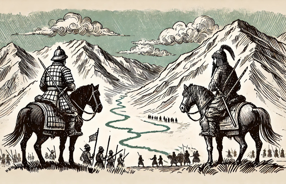
Imagine two generals, a “Defender” (Li) and an “Attacker” (Gar). To embed the story into a semi-historical context, one can picture the dilemmas of the generals and emperors from the Tang-Tibetan Wars in the 7th century. (The Himalayas or other mountains of Central Asia and the Tibetan Plateau could provide the mountain scene.) Li and Gar are preparing for battle near a mountainous region more than a thousand years ago – in an era when technology for reliable weather forecasting was not accessible. The possible battlegrounds are new for both generals, but scouts identified two directions for the attack – an upper route in the hills and a lower route in a valley. In the hills, the ever-changing weather also plays a crucial role. By a sudden storm, it can wipe out a whole attacking army.
Both generals can choose from two actions. Li can decide to defend the upper or the lower route, while Gar can decide to attack from the same two directions. The next day, the weather can be in two states; there can be a storm in the hills, or the weather can stay calm.
The winning and losing prospects depend on the actions of the generals and on the weather in the following way: If the weather is calm, then Li loses if he is attacked from an undefended direction, but the defence is always successful if both generals choose the same direction. In case of a storm, however, the attacking army would be lost if it dared the upper route. (On the lower route, in the valley, the weather does not change the outcome of a battle.)
The winning and losing prospects depend on the actions of the generals and on the weather in the following way: If the weather is calm, then Li loses if he is attacked from an undefended direction, but the defence is always successful if both generals choose the same direction. In case of a storm, however, the attacking army would be lost if it dared the upper route. (On the lower route, in the valley, the weather does not change the outcome of a battle.)
Assuming that no general has reliable knowledge about the weather or can reliably associate a probability distribution to it – and their lack of information is common knowledge – what strategy should the generals follow? (The generals are capable of randomization – methods such as divinations of various kinds were used from prehistory to make randomized actions.)
(Illustartion generated by DALL·E at 2025. 03. 07. )
Winning and losing probabilities can be represented by two-by-two utility matrices. Rows represent the actions of Player 1 (the Defender) while columns represent the actions of Player 2 (the Attacker). Both have two choices, going on the upper or lower route ).
(=={"Up","Down"}
1
2
In[]:=
MatrixForm[u1["Calm"]={{1,0},{0,1}}]MatrixForm[u1["Storm"]={{1,0},{1,1}}]
Out[]//MatrixForm=
1 | 0 |
0 | 1 |
Out[]//MatrixForm=
1 | 0 |
1 | 1 |
In[]:=
MatrixForm[u2["Calm"]=1-u1["Calm"]]MatrixForm[u2["Storm"]=1-u1["Storm"]]
Out[]//MatrixForm=
0 | 1 |
1 | 0 |
Out[]//MatrixForm=
0 | 1 |
0 | 0 |
In[]:=
U1={u1["Calm"],u1["Storm"]}U2={u2["Calm"],u2["Storm"]}
Out[]=
{{{1,0},{0,1}},{{1,0},{1,1}}}
Out[]=
{{{0,1},{1,0}},{{0,1},{0,0}}}
For this representative case the Extended Equilibrium can be computed, yielding the following parameters:
◼
p - the probability that Player 1 (the Defender) will choose the first action (defending the upper route),
◼
q - the probability that Player 2 (the Attacker) will choose the first action (attacking the upper route),
◼
P - the emergent subjective prior of Player 1 (the Defender) that the deeply unknown parameter will be in the first state (i.e. the weather will be calm),
◼
Q - the emergent subjective prior of Player 2 (the Attacker) that the deeply unknown parameter will be in the first state (i.e. the weather will be calm).
In[]:=
pqPQ=MinimalUncertaintyGameSolve[〈U1,U2〉]
Out[]=
p1-,q2-,Q-1+
1
2
2
,P1
2
2
In[]:=
pqPQ//N
Out[]=
{{p0.292893,q0.585786,P0.707107,Q0.414214}}
In[]:=
ρ={〈{"p",1-"p"},{"q",1-"q"}〉,〈{"P",1-"P"},{"Q",1-"Q"}〉}/.pqPQ[[1]]
Out[]=
1-,,2-,1-,-1+
1
2
1
2
2
,-1+2
,1
2
1
2
2
,2-2
Comparison with Bayesian Games
Comparison with Bayesian Games
If we assume that both generals have the same common prior about the weather, then the problem can be formulated as a Bayesian or Harsányi game. In this simple case, this Bayesian game can be represented as a set of zero-sum games, parametrized by one parameter – the commonly believed probability of Calm weather – P.
In the Wolfram Language, such parameter-dependent games can be natively defined and manipulated:
In the Wolfram Language, such parameter-dependent games can be natively defined and manipulated:
(*Inthedefinitionweneedtoconverttheutilitymatricesfrom"Component Arrays"to"Composite Arrays"*)BGWgame[P_]:=MatrixGame[Transpose[{u1["Calm"]P+u1["Storm"](1-P),u2["Calm"]P+u2["Storm"](1-P)},RotateRight[Range[3]]],GamePlayerLabels{"Defender","Attacker"},GameActionLabels{{"Up","Down"},{"Up","Down"}}]BGWgame[2/3]["Dataset"]
Out[]=
|

In[]:=
MatrixGamePlot[BGWgame[2/3]]
Out[]=
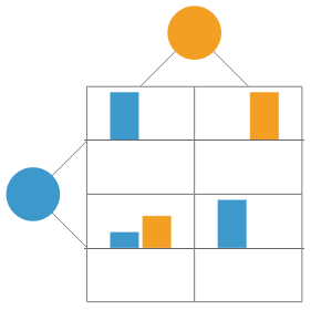


If, for example, the commonly believed prior for a calm weather is P = 2/3, then we get the following equilibrium strategies for the generals:
In[]:=
FindMatrixGameStrategies[BGWgame[2/3]]
Out[]=
,,,
2
5
3
5
3
5
2
5
BpqList=Table[{P,FindMatrixGameStrategies[BGWgame[P]][[1,;;,1]]},{P,1/100,1,1/100}];
In[]:=
ListLinePlot[{{#[[1]],#[[2,1]]}&/@BpqList,{#[[1]],#[[2,2]]}&/@BpqList},PlotLegends{"p(P)","q(P)"},AxesLabel{"P","p/q"}]
Out[]=
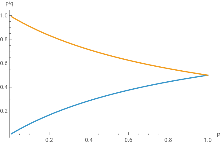


However, if we plot together the possible equilibrium values for these Bayesian games and the equilibrium values obtained by the Extended Equilibrium on the “p”-“q” plane, then we need to conclude that no common prior corresponds to the previously calculated equilibrium strategy.
In[]:=
ShowListLinePlot[{#[[2,1]],#[[2,2]]}&/@BpqList,PlotRange{{0,1},{0,1}},AxesLabel{"p","q"},AspectRatio1],GraphicsPoint1-1√2,2-√2
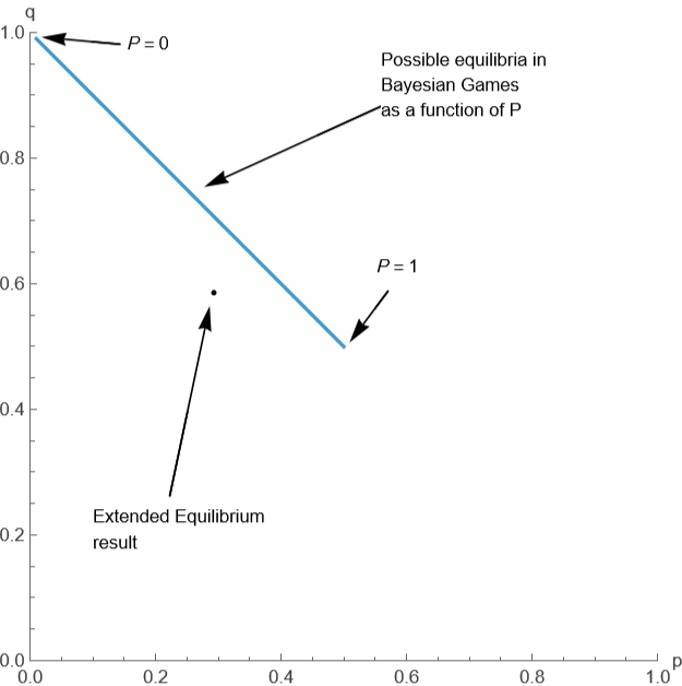
This example directly shows that handling parameter uncertainty with the concept of Extended Equilibrium differs and goes beyond the framework of Bayesian or Harsányi games.
(For more detailed analysis, see Subsection 6.0.1 in the paper.)
(For more detailed analysis, see Subsection 6.0.1 in the paper.)
Coordination Game with Uncertain Payoffs
Coordination Game with Uncertain Payoffs
Solving a version of the Battle of the Sexes game (also known as Bach or Stravinsky game), where the payoffs (or more precisely the utilities) depend from an uncertain parameter:
Providing an example, where multiple Extended Equilibria exist.
Removal of the package
Removal of the package
To reload the package you might use the following Get[] to avoid potential ::shdw errors.
Acknowledgements
Acknowledgements
Besides friends and colleagues mentioned in the paper's final section, I owe special thanks and am very grateful to Ahmed Elbanna from Wolfram Research for his help in formatting and publishing the present post.
CITE THIS NOTEBOOK
CITE THIS NOTEBOOK
Non-cooperative games with uncertainty
by József Konczer
Wolfram Community, STAFF PICKS, January 9, 2026
https://community.wolfram.com/groups/-/m/t/3604012
by József Konczer
Wolfram Community, STAFF PICKS, January 9, 2026
https://community.wolfram.com/groups/-/m/t/3604012