Fusible numbers are a set of rational numbers that can be constructed through a simple binary operation: x ∼ y. As will be illustrated, this simple setup yields rich algebraic and (transfinite) combinatorial structures [3]. Moreover, two of the most intriguing aspects pertaining to our study of fusible numbers, are first, their well-ordering (by an order type of) that in turn allows the construction of useful algorithms in studying their properties (by exploiting that well-orderdness). Second, fusible numbers can be represented as pure binary trees which makes expressing and manipulating them in Schönfinkel’s combinator form possible. Moreover, we see that the fuse operation is an example of a fast-growing function in combinatorics that similar to Goodstein’s sequence and the Ackermann function is independent of Peano arithmetic due to its unique properties.
ε
0
1. From the riddle to its formal definitions
1. From the riddle to its formal definitions
1.1. The mathematical riddle
1.1. The mathematical riddle
Fusible numbers have simple beginnings. It started with the work of Ericson [1]; he wanted to formalize the following mathematical riddle of measuring different amounts of time by the act of lighting fuses:
'You are given two fuses: x and y. Each one burns for exactly 1 minute, but does so irregularly, so one cannot know exactly how much of the fuse has been burnt up after a given amount of time by just measuring it's length after a period of time. Rules: you are allowed to light one or more unlit ends of any fuse, but only at time 0 or when a fuse burns out completely. How do you measure 45 seconds? '
The solution is to light three ends at t=0: two ends of fuse x and one end of fuse y. When the fuse x burns out completely from the both ends, 30 seconds have passed —at that instant, light the remaining end of the fuse y. Forty-five seconds will have passed when the fuse y burns out. On that basis, we can ask: what other numbers can we get to by the simple fuse operation x ∼ y besides 0, 1/2, 3/4? This is the essence of fusible numbers.
1.2. The formal definitions
1.2. The formal definitions
◼
Fusible numbers are a set of nonnegative numbers in , that have an order type of an ordinal.
ε
0
◼
Fusible numbers are both well-ordered and closed under addition.
◼
All fusible number are also dyadic rationals whose denominator is a power of 2.
◼
All fusible numbers can be 'fused' together from 0 with the binary fuse operation, namely x ∼ y over the real numbers with the following restriction: |x-y| < 1 as x and y, the two fusible numbers, cannot have a difference greater than 1 (time) unit between them.
=
x+y+1
2
2. The fuse operation in action
2. The fuse operation in action
Here, the consequences, the repeated application of the fuse operation x ∼ y = where |x-y| < 1, gives rise to, will be explored.
=
x+y+1
2
2.1. Generating fusible numbers
2.1. Generating fusible numbers
For starters, let’s ‘fuse’ together some numbers:
(Debug) In[]:=
(*generatingfusiblenumbers*)cond[a_]:=Abs[a[[2]]-a[[1]]]<1sim[a_,b_]:=(a+b+1)/2nextFusibles[fusiblesIn_]:=Module[{t,newFusibles},t=Select[Tuples[fusiblesIn,5],cond];newFusibles=Table[sim[t[[i,1]],t[[i,2]]],{i,1,Length[t]}];DeleteDuplicates[Join[fusiblesIn,newFusibles]]]
(Debug) In[]:=
Nest[nextFusibles,{0},5]
(Debug) Out[]=
0,,,1,,,,,,,,,,,,,,,,,2,,,,,,,,,,,,,,,,,,,,,,,,,,,,,
1
2
3
4
7
8
9
8
5
4
11
8
3
2
15
16
19
16
21
16
23
16
25
16
13
8
27
16
7
4
29
16
15
8
31
16
31
32
39
32
43
32
45
32
47
32
49
32
51
32
53
32
55
32
57
32
59
32
61
32
63
32
65
32
33
16
67
32
17
8
69
32
35
16
71
32
9
4
73
32
37
16
75
32
19
8
77
32
39
16
79
32
5
2
2.2. Growth in the density of fusible numbers
2.2. Growth in the density of fusible numbers
The density of fusible numbers along the real line grows at a very fast rate:
Erickson et al . [1] Theorem 1.2. Let g(n) be the largest gap between consecutive fusible numbers in F ∩[n, ∞). Then ≥ F(n − 7) for all n≥8, where F denotes the fast-growing hierarchy.
-1
g(n)
ε
0
ε
α
(Debug) In[]:=
(*thisvisualizesthedenisityoffusiblenumbers*)Nest[nextFusibles,{0},10]//Graphics[{Line[{{#,0},{#,1/8}}]&/@#},Axes->{True,False},PlotRange->{{0,4},All},ImageSize->10×72,AspectRatio->1/10]&
(Debug) Out[]=
◼
line snippet showing the density of fusible numbers (identical-looking graph to Ericson et al.[1])
We observe that the growth in the density of fusible numbers is not monotonous. After the first few fusible numbers, their density starts to exhibit an incredibly rapid growth (at least like the functionFε₀ of the fast-growing hierarchy [1]) but it does so irregularly: increasing around accumulation points to where they converge, after which their density drops sharply.
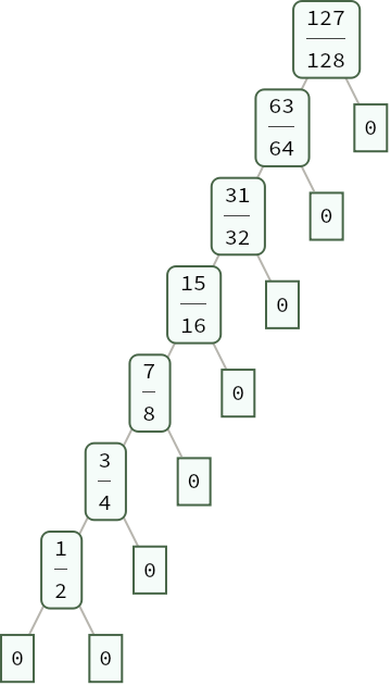
Let’s first consider all the fusible numbers 0 ≤ x ≤ 1. The first three being 0, 1/2 and 3/4 (the one’s included in the riddle). We can continue generating new numbers by repeatedly applying the fuse operation e.g. by lighting more and more consecutive fuses, in other words adding ∼ 0 to the existing fusible numbers, starting from zero; in doing so we generate infinitesimally smaller numbers:
0∼0=1/2, 1/2∼0=3/4, 3/4∼0=7/8, 7/8∼0=15/16, 15/16∼0=31/32, 31/32∼0=63/64, 63/64∼0=127/128...
◼
the corresponding linear tree structure: applying the ∼ 0 operation
More generally, all fusible numbers <1 have the form for n ∈ N:
1-
-n
2
(Debug) In[]:=
ClearAll[fusibleN];fusibleN[b_]:=1-;
-1-(b-2)
2
(Debug) In[]:=
fusibleN[Range[25]]
(Debug) Out[]=
0,,,,,,,,,,,,,,,,,,,,,,,,
1
2
3
4
7
8
15
16
31
32
63
64
127
128
255
256
511
512
1023
1024
2047
2048
4095
4096
8191
8192
16383
16384
32767
32768
65535
65536
131071
131072
262143
262144
524287
524288
1048575
1048576
2097151
2097152
4194303
4194304
8388607
8388608
16777215
16777216
fusibleN[b_]:=1-;
-1-(b-2)
2
As demonstrated, this sequence converges to 1. In fact, there are infinitely many fusible numbers that are less than 1, let’s take the 10^3/2th:
(Debug) In[]:=
Block[{$RecursionLimit=10^4},RepeatedTiming[fusibleN[10^3/2]]]
(Debug) Out[]=
{8.42115×,16366953039480709350065948484137995761083210230215323947416456840480668982023372774416350461629520785754433420637800355046086282729426965266642637946871636695303948070935006594848413799576108321023021532394741645684048066898202337277441635046162952078575443342063780035504608628272942696526664263794688}
-6
10
(Debug) In[]:=
N[Last[%],155]
(Debug) Out[]=
0.999999999999999999999999999999999999999999999999999999999999999999999999999999999999999999999999999999999999999999999999999999999999999999999999999999389013
2.2. Limit ordinals: from ω to ε0
2.2. Limit ordinals: from ω to
ε
0
◼
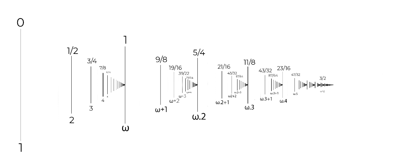
fusible numbers from 0 to 3/2 and their corresponding ordinals up to a double limit point at.
2
ω
Part of Erickson et al . [1] Theorem 1.1. The set of fusible numbers, when ordered by the usual order “ < “ on R, is well-ordered with an order type of .
ε
0
As a consequence of their well-orderdness, we are able map fusible numbers to the ordinals in way that is uniquely order-preserving. Therefore, 1, to which our first infinite sequence of fusible number converges, behaves like the smallest transfinite ordinal ω. We reach more of these accumulation points by repeatedly ‘fusing’ together more and more numbers, e.g. we now apply ∼1/2 to the existing fusible numbers that lie between 1/2 and 1 :
1∼1/2=9/8, 9/8∼1/2=19/16, 19/16∼1/2=39/32, 39/32∼1/2=79/64, 159/128∼1/2=319/256, 319/256∼1/2=639/512, 639/512∼1/2=1279/1024...
1∼1/2=9/8, 9/8∼1/2=19/16, 19/16∼1/2=39/32, 39/32∼1/2=79/64, 159/128∼1/2=319/256, 319/256∼1/2=639/512, 639/512∼1/2=1279/1024...
Consequently, our next accumulation point is at 5/4 to which the above sequence converges. 5/4 behaves like ordinal 2ω; the fusible numbers in that region are of the form for n ∈ N:
5/4-1-
-n
2
(Debug) In[]:=
fusibleN2[b_]:=5/4-;fusibleN2[Range[0,15]]
-1-(b+1)
2
(Debug) Out[]=
1,,,,,,,,,,,,,,,
9
8
19
16
39
32
79
64
159
128
319
256
639
512
1279
1024
2559
2048
5119
4096
10239
8192
20479
16384
40959
32768
81919
65536
163839
131072
Also, for 11/8 (3ω) the fusible numbers between 5/4 and 11/8 have the formula for n ∈ N
11/8-1-
-n
2
(Debug) In[]:=
fusibleN3[b_]:=11/8-;fusibleN3[Range[10]]
-1-(b+1)
2
(Debug) Out[]=
,,,,,,,,,
5
4
21
16
43
32
87
64
175
128
351
256
703
512
1407
1024
2815
2048
5631
4096
These limit points all converge to 3/2: a 'double limit point ', which we can associate with:
2
ω
(Debug) In[]:=
fusibleN4[b_]:=3/2--;fusibleN4[Range[10]]
-(b+1)
2
-(b+1)
2
◼
an updated graphic with some transfinite ordinals
2.3. An algorithm that translates a fusible number to its ordinal, vice-versa
2.3. An algorithm that translates a fusible number to its ordinal, vice-versa
2.3.1. Integer fusible numbers
2.3.1. Integer fusible numbers
◼
this algorithm works for all the fusible numbers until ε₀
2.3.2. From ordinals to fusible numbers
2.3.2. From ordinals to fusible numbers
In section 2.2 we used separate formulae for calculating the sequences of fusible numbers; there were discontinuities in these sequences due to accumulation points; this makes the pairing the two representations difficult.
The following function is an example of transitioning between fusible numbers and their corresponding ordinals. It is a low-yielding one, however, as it only finds corresponding fusible numbers between the lowest transfinite ordinal ω and the second ω2, e.g. when inputting ω+299792458, it outputs the corresponding fusible number. Ideally one wants a a more general formulae for calculating the sequences of fusible numbers in different sections along the real line.
2.4. The recursive algorithm: finding successive fusible numbers
2.4. The recursive algorithm: finding successive fusible numbers
Again, based on the well-ordering principle, Xu et al., on that basis, have defined the following recursive algorithm that allows us to find fusible numbers greater than x .
Through implementation,
we can compute both m(x): giving us the smallest distance to the next fusible number and s(x): the smallest fusible number over that distance. As highlighted, this recursive algorithm is prone to fail sooner or later given the incredibly fast-growing nature of the fuse operation:
One point to add, anything above m(2) took simply too long to calculate: following function shows the recursive calls made by m(x). This implies the inefficiency of m(x). We also considered finding a non-recursive algorithm that would overcome the computational costs associated with it, but were unsuccessful.
◼
recursive calls made by the algorithm m(x) for m(2)
2.5. Algorithm for deciding whether a given number is fusible
2.5. Algorithm for deciding whether a given number is fusible
Additionally, one of the tasks of this project was to create an algorithm FusibleQ that decides whether a number is fusible or not. For starers, an obvious criteria that tests for ‘fusibility’ is to consider only dyadic rationals as potential candidates. Nevertheless, the trouble with finding a general formula, is that, by definition we have an infinite collection of fusible numbers all of which can go into constructing that particular fusible number that we are testing the ‘fusibility’ on. That property makes these types of computations difficult. The same notion also became an obstacle in the section 3.2 whilst creating an algorithm that deconstructs fusible numbers into its component parts.
3. Individual fusible numbers
3. Individual fusible numbers
Subsection 3.1. Representing fusible numbers as binary trees
Subsection 3.1. Representing fusible numbers as binary trees
◼
a few random combinations for 43/32, showcasing ‘binary branching’
Nevertheless, every fusible number has a maximum-height representation; otherwise the well-ordering principle would not hold. What follows, are some 'snapshots' of fusible numbers, based on the number of leaves.
3.2. Deconstructing fusible numbers to its minimal binary tree compositions
3.2. Deconstructing fusible numbers to its minimal binary tree compositions
Some examples on the basis of which the algorithm was built:
◼
5/4 should generate two decompositions
◼
the first pair is rejected as their difference is greater than 1
◼
the first three are rejected as their differences are greater than 1
◼
integers
Overall, the algorithm does what it is supposed to do, reducing fusible numbers to their minimal component parts. However, there are some minor issues: 5/4 seems to be a problem; when doing the decomposition, we only find one of the partitions that work, the other partition needs to be tweaked: the rational number needs to be changed from 3/4 to 6/8 in order for the decomposition to work.
4. Fusible number-combinator connection
4. Fusible number-combinator connection
◼
1/2= (0 ∼ 0) and 1=(0 ∼ 0) ∼ (0 ∼ 0)
Moreover, as already showcased, the same fusible numbers can have differing structures. In the zero-tilde notation, 3/4 can be represented either as (0~0)~0 or 0~(0~0)
In using the zero-tilde notation, we’ll try to use S-combinators to generate fusible numbers.
5. Plotting all the ‘fusion’ events
5. Plotting all the ‘fusion’ events
Subsection 5.1. The token-event graph
Subsection 5.1. The token-event graph
Now we generate all the possible combinations of fusible numbers in the confines of a reasonable number of time-steps. First, we have plotted the results onto a simple nested graph that has tokens in the middle. These tokens act as disambiguation by showing how the precursor numbers are fed in pairs to create the new numbers through the fuse operation; whereas the actual nodes of the graph are the fusible numbers themselves. Therefore, our nested graph was split into two classes:
◼
the first few ‘fusion’ events
◼
continuing for longer we get a more complex structure:
The result is a widening DAG-graph, showing the possible ‘fusion’ events; how the fusible numbers are created and related to each other. The total number of distinct numbers reached is relatively high, but for a more thorough analysis more time-steps need to be performed.
The graph that follows, has been run for more time steps and has had events removed; only showcasing all the possible fusible numbers generated.
◼
A token-graph showing the behaviour of fusible numbers; here the 0, from where ‘fusing’ begins, is at the bottom.
Conclusion
Conclusion
Whereas the complex proofs underlying fusible numbers can be found elsewhere [1], this simple computational study, was still fruitful in providing nice insights into the behavior of fusible numbers and was a rare example of having to use transfinite numbers in problem solving. There are still plenty loose ends and our preliminary analysis leaves room for many extensions:
◼
We found a few inconsistencies in the decompositions/partitions of fusible numbers; the algorithms needs tweaking
◼
Transitioning from ordinals to fusible numbers and vice versa, was very limited and a more general formulae would be needed.
◼
One could also consider finding a non-recursive algorithm for m(x).
◼
A spin-off project would be implement ordinal/transfinite arithmetic in Mathematica, given the lack functionalities associated with it, that we came across during this project.
Keywords
Keywords
◼
token-event graph
◼
binary tree
◼
transfinite numbers
◼
ordinals
◼
combinators
◼
fast-growing functions
Acknowledgment
Acknowledgment
I would like to thank my mentor, Bob Nachbar for his mentorship, thanks to him, Wolfram Summer School has been a very rewarding experience for me. I would also like to thank Michael Reed, Christopher Wolfram and Daniel Robinson for their insights and of course, Stephen Wolfram, for the advice that he gave me during the meetings at the Summer School.
References
References
◼
[1] J. Erickson, G. Nivasch, and J. Xu. Fusible numbers and Peano Arithmetic. 2020. arXiv: 2003.14342
◼
[2] Ryu Hasegawa. Well-ordering of algebras and Kruskal’s theorem. In N. D. Jones, M. Hagiya, and M. Sato, editors, Logic, language and computation, volume 792 of Lecture Notes in Computer Science, pages 133–172. Springer, 1994.
◼
[3] J. Xu. Survey on fusible numbers. 2012. arXiv: 1202.5614