Step by step description of how to generate and interpret the most commonly used aircraft performance charts. Not peer reviewed. These are notes from the presentation: Phantoms, MiGs, and Kinematics: The Math of Dogfighting, Wolfram Virtual Technology Conference, November 5-7, 2025A
Function Declaration
Modeling Aircraft Performance
The Standard Atmosphere Model
The Standard Atmosphere Model
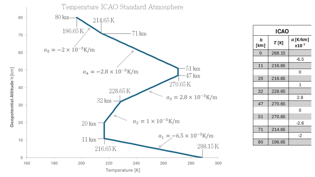
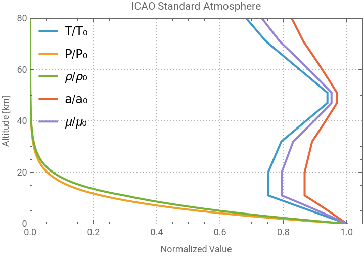
A function of the International Standard Atmosphere (ICAO, 1993 [1]) is first defined to model the changing atmospheric conditions at every altitude. The model is divided in isothermal and layers with temperature gradient a. Please see the reference for the complete equations, the following figure can be used as a guide:The following figure describes the normalized behaviour of the most important thermodynamic properties.
In[]:=
ISAPlot[80000] (*up to 80 km -> 80000 m*)
Out[]=
Aircraft Definition
Aircraft Definition
McDonell-Douglass F-4 Phantom II
McDonell-Douglass F-4 Phantom II
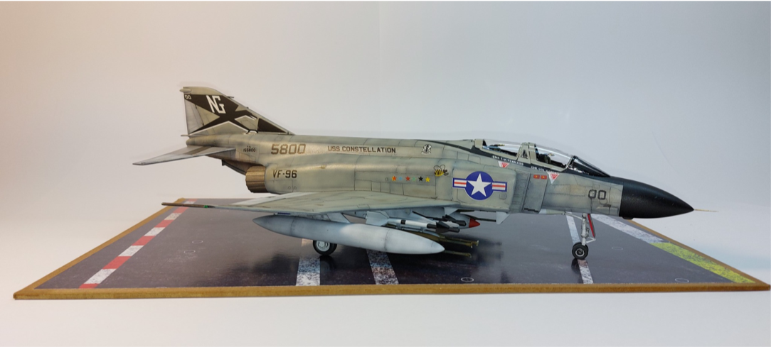
The F-4 Phantom was the premier fighter aircraft from the Cold War. With its twin-engine, twin seat all-weather long-range interceptor and fighter bomber with service in the United States Air Force (USAF), the U. S. Marine Corps and the U.S. Navy. Below is a photo of a 1/48 plastic scale model built by the author with the livery of Randall “Duke” Cunningham, the first U.S. Navy ace of the conflict. The information comes from multiple open sources and was calibrated based on published data.
F-4 Phantom II Data Association
F-4 Phantom II Data Association
Mikoyan-Gurevich Mig 21
Mikoyan-Gurevich Mig 21
Drag Estimation
Drag Estimation
Forces on an airplane
Forces on an airplane
Subsonic drag
Subsonic drag
Supersonic drag modelling
Supersonic drag modelling
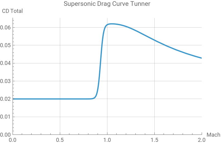
The supersonic drag (wave drag) is much more complex to model. It is the drag created by the shock waves on an airplane crossing near and after the speed of sound. The approach to modelling this is based on the equations developed by Krus & Abdallah (2019) [b]. It is a mathematical manipulation of the famous Prandtl-Glauert correction so that it does not get undetermined at Mach=1. By the use of shaping factors kwd, kdwm, Mcrit and dragIncrease, one shapes the Mach to match the experimental data shown on flight reports using a sigmoid curve. The equations are given here and the Manipulate graph is used to shape these curves. The reader is invited to consult the full paper for details
C
D
wave
1
1+
-9
M-(1-/2)
δ
M
δ
M
e
k
dw
4
2
(M-)
k
dwm
4
k
dw
Where: dragIncrease = Shaping factor [ ] = (1-) = Aircraft critical Mach Number [ ] = Shaping factor [ ] = Shaping factor [ ]
δ
M
M
crit
M
crit
k
dw
k
dwm
The following graph shows how these factors affect the shape of the wave drag, and all of these equations are included in the EstimateDrag function.
Out[]=


Drag vs. Mach plot
Drag vs. Mach plot
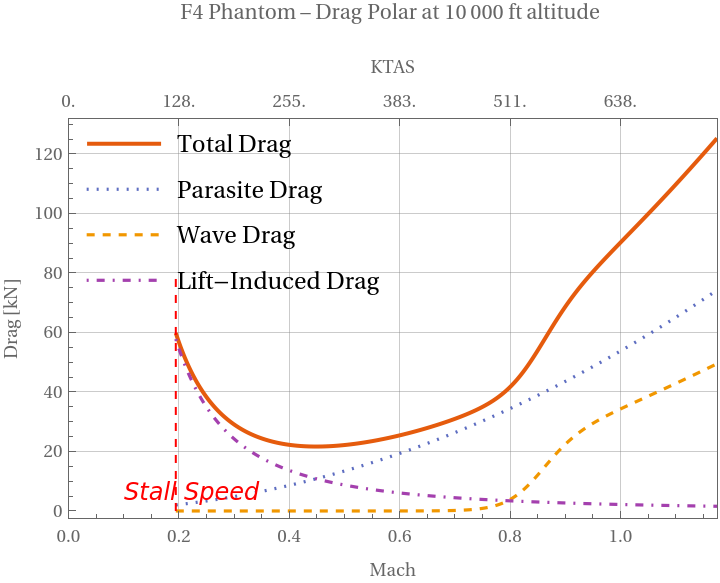
The drag force as a function of speed is plotted on the next graph for the Phantom. It can be seen that the parasite drag increases with velocity, while the opposite happens to the induced drag. The wave drag (due to supersonic effects) starts to rise even before reaching supersonic speeds (at transonic speeds of ~0.77 Mach, which is the ), when compressibility effects begin to occur. This generates a small “bump” close to Mach 1.
M
crit
In[]:=
(* Sending [airplane, altitude,min Mach,max speed in knots]*)DragPolarMach[F4PhantomDataSI,10000,0.1,750]
Out[]=
Maximum endurance and maximum range speeds for a jet
Maximum endurance and maximum range speeds for a jet
Aerodynamic efficiency (L/D)
Aerodynamic efficiency (L/D)
Glide polar
Glide polar
Thrust and Power
Thrust and Power
Thrust modelling
Thrust modelling
The job of aircraft jet gas turbine engines is to provide thrust to the airplane to allow it to accelerate through the air. Aircraft aero engines are one of the most complex engineering systems ever made, and therefore for preliminary performance estimations, a model with major simplifications is needed. The following equation is used to model the engine thrust as a function of altitude. The engine thrust The engine thrust is equal to the sea-level static thrust (), scaled by the ratio of local to sea-level air density and further reduced by a linear Mach-number factor that decreases thrust by 25 % per unit Mach. This accounts for the reduced thrust as foreward speed increases due to compressibility effects, intake losses, compressor efficiency, etc. This model was obtained from [c]. Where: T = Thrust [N] = Sea-level static thrust [N] ρ= Air density at altitude[kg/m3] =Air density at sea level[kg/m3] = Mach [ ]The following plot shows the thrust available () and total drag ()as a function of Mach and speed. The intersection point between the curves (where = ) is the maximum achievable speed of the airplane in level flight. The engine cannot produce more thrust to overcome the drag and therefore cannot accelerate any more. The area between the curves has the units of Power since Force Velocity = Power [W]
T
0
ρ
ρ
0
T=(1-0.25M)
T
0
ρ
ρ
0
T
0
ρ
0
M
T
ava
D
tot
T
ava
D
tot
∫(-)V=∫ForceV
T
ava
D
tot
Power curves
Power curves
Specific Excess Power
Specific Excess Power
Vy and Vx speeds
Vy and Vx speeds
SEP Contour Plots
SEP Contour Plots
Modifying the previous diagram for different altitudes will show that the SEP changes not only depending on velocity, but also on altitude.
Because SEP depends on both altitude and speed, we can calculate it over a range of Mach numbers and altitudes. The following function computes the SEP values for every combination of altitude and speed, and stores the results as a set of {altitude, velocity, SEP} data points.
This behavior can be visualized on a 3D surface plot, where the mesh lines represent constant SEP values. The plot shows that the highest SEP values (in red) occur near sea level, and gradually decrease with increasing altitude until eventually the SEP reaches zero. This point marks the aircraft’s absolute ceiling, where there is no excess power available to sustain a climb. At the SEP=0 condition, power available equals the power required.
If the 3D SEP surface is viewed from above, one sees the following:
Going from 3D to 2D can be done using a contour plot, the result is the following figure, where Mach is shown on the x-axis and altitude on the y-axis.
This analysis showing the energy state of the aircraft and its capacity to accelerate or climb is the foundation of the mathematical modelling of a dogfight.
Energy Maneuverability Chart
Energy Maneuverability Chart
Introduction
Introduction
Agility
Agility
This so-called “doghouse diagram” has information about agility. This is defined as the ability to make rapid, controlled changes in airplane motion, which include climb, acceleration, deceleration, and turn characteristics. The ability to make rapid changes describes maneuverability; the ability to precisely guide the airplane through such changes describes controllability. Thus, maneuverability and controllability are subsets of agility.
Forces in a turn
Forces in a turn
Turn rate and Turn Radius
Turn rate and Turn Radius
Aircraft limits
Aircraft limits
Aerodynamic limit
Aerodynamic limit
Structural limits
Structural limits
Specific Excess Power
Specific Excess Power
Equations used
Equations used
Model analysis
Model analysis
Model comparison
Model comparison
Aircraft comparison
Aircraft comparison
References
[0] Pedersen, D. (2022). TOPGUN: The Real Story. Penguin Books Ltd.
[1] Boyd, J. R. (1964). Aerial attack study (rev. Jan. 4, 2016 ed.). Nellis Air Force Base; reproduced by Code 7700. https://code7700.com/pdfs/john_boyd/aerial-attack-study-1964_john_boyd.pdf
[a] International Civil Aviation Organization. (1993). Manual of the ICAO standard atmosphere: Extended to 80 kilometres (262,500 feet) (3rd ed.). ICAO. Retrieved September 30, https://news.ncac.mn/uploads/bookSubject/2022-11/6369ec174ab34.pdf
[b] Krus, Petter & Abdallah, Alvaro. (2019). Modelling of Transonic and Supersonic Aerodynamics for Conceptual Design and Flight Simulation. 30-34. 10.3384/ecp19162003.
[c] Staack I and Franzen L K. Aircraft and Vehicle Design. 6, v2023 ed. TMAL02 Course Material, Linköping University, Sweden, 2023.
[d] Ruijgrok, G. J. J. (2009). Elements of airplane performance (2nd ed.). VSSD. https://resolver.tudelft.nl/uuid:9ff3c7e0-e221-4d8f-bf9e-e144d3cacdc1
AI usage
AI usage
During the preparation of this work the author used ChatGPT 5 in order to generate and modify Wolfram Language Code. After using this tool/service, the author reviewed and edited the content as needed and takes full responsibility for the content of the presentation.
Licence
Licence
CITE THIS NOTEBOOK
CITE THIS NOTEBOOK
Phantoms, MiGs, and kinematics: modelling energy-maneuverability diagrams
by Erick Espinosa-Juárez
Wolfram Community, STAFF PICKS, February 13, 2026
https://community.wolfram.com/groups/-/m/t/3639758
by Erick Espinosa-Juárez
Wolfram Community, STAFF PICKS, February 13, 2026
https://community.wolfram.com/groups/-/m/t/3639758